
I’ve been messing around with LLM pre-training, seeing how much I can squeeze out of limited compute. Most people training language models from scratch do the same thing: stack some Transformer blocks, throw AdamW at it, maybe add flash attention. Works fine, but it’s boring.
I got curious about borrowing ideas from computer vision. U-Net’s skip connections translated better to language models than I expected.
Why U-Net?
U-Net’s everywhere in computer vision. Originally built for biomedical image segmentation, now it’s the go-to architecture for anything with spatial hierarchies. The idea is skip connections: early layers catch fine details, later layers catch the big picture, and you mix them together.
Language has hierarchies too. Characters build into words, words into phrases, phrases into sentences. I figured the skip connection pattern might work on a Transformer.
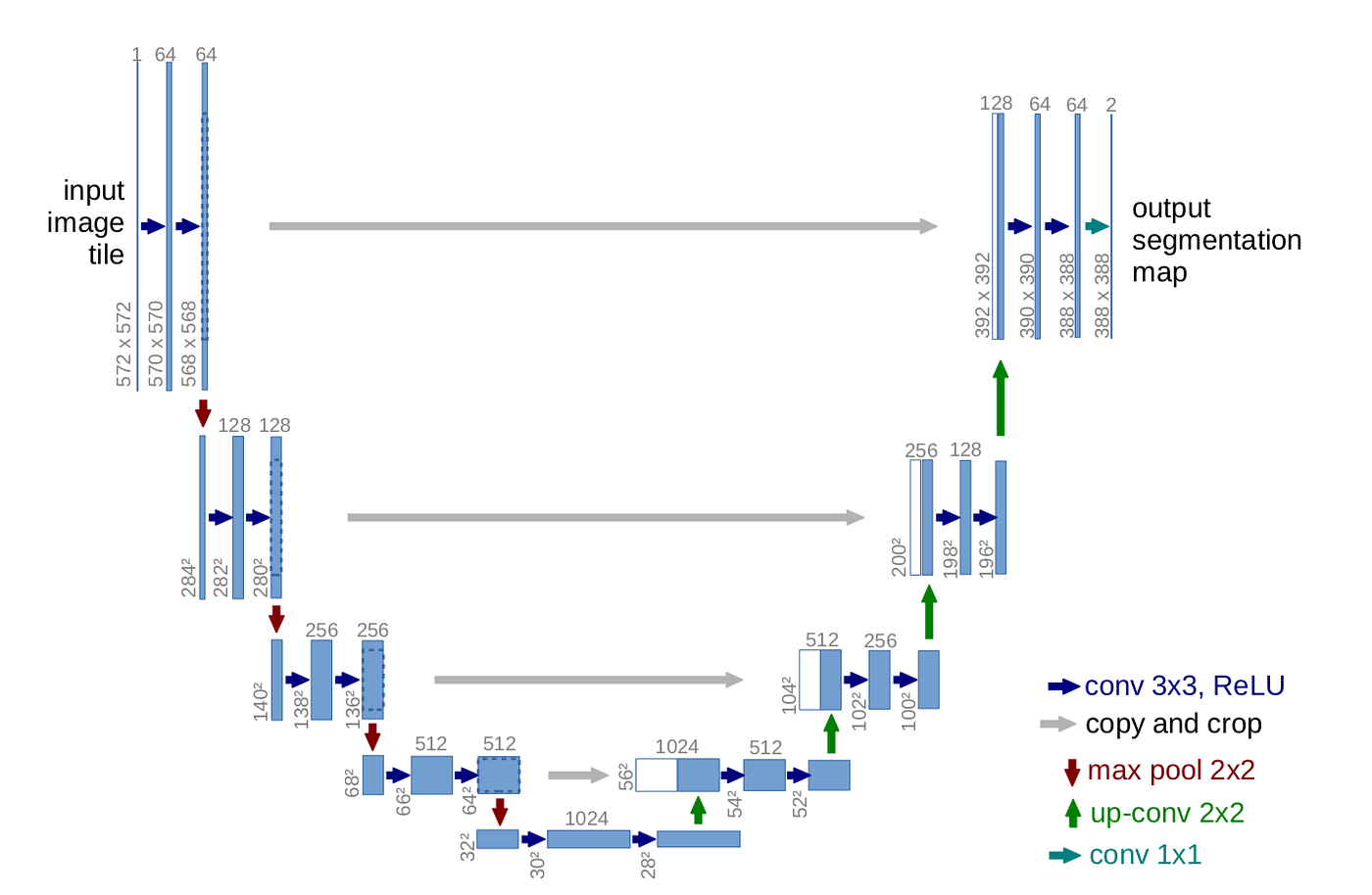
The setup is straightforward. 16 Transformer layers, split in half: layers 1-8 store their activations (the “down” path), and layers 9-16 mix those stored activations back in via learned gates (the “up” path).
Each gate is just a parameter per dimension, starts at 0.1. The mixing formula couldn’t be simpler:
\[\text{output} = \text{gate} \times \text{skip} + (1 - \text{gate}) \times \text{current}\]
The network learns how much to rely on earlier features versus later ones. In practice, I found the gates converge to different values per layer. Some rely heavily on skip connections (gate ≈ 0.7), others barely use them (gate ≈ 0.1).
Here’s the core implementation:
1 | class GatedMixer(nn.Module): |
The training loop stores activations from the first 8 layers, then mixes them into the upper 8 layers in reverse order. Layer 9 gets mixed with layer 8’s output, layer 10 with layer 7, and so on.
Not All Layers Are Equal
Something became obvious during training: not all layers need the same attention mechanism. Early layers care about local patterns, like what words are next to each other and basic syntax. Later layers need context, like what the whole sequence is trying to say.
For layers 1-8, I used sliding window attention. Standard multi-head attention with a 256-token window, borrowed from Longformer. Only attend to nearby tokens, saves memory, makes sense for local patterns.

Token at position \(i\) can only see \([i - 256, i]\). You lose some long-range dependencies, but that’s fine. We’re building up local representations first. The global view comes later.
For layers 9-16, I switched to Multi-Query Attention (MQA). Instead of each attention head getting its own key and value projections, they all share one K and one V. Sounds weird, but it works. The KV cache shrinks dramatically, which matters for inference.

With 8 heads and d_model=1024, standard MHA needs 8
separate K/V projections (128 dims each). MQA shares one K and one V
across all heads. For 512 tokens, that’s roughly 8× less KV cache
memory.
Both attention types use RoPE for positional embeddings. Instead of adding position encodings to the input, it rotates Q and K vectors based on position. The nice thing about RoPE is that relative positions get encoded in the dot product itself.

The rotation is computed using sine and cosine functions:
\[\text{freq}_{j} = \frac{1}{10000^{2j/d}}\]
\[\text{RoPE}(x, \text{pos}) = \begin{pmatrix} x_{1} \\ x_{2} \\ \vdots \end{pmatrix} \odot \begin{pmatrix} \cos(\text{pos} \cdot \text{freq}) \\ \cos(\text{pos} \cdot \text{freq}) \\ \vdots \end{pmatrix} + \text{rotate\_half}(x) \odot \begin{pmatrix} \sin(\text{pos} \cdot \text{freq}) \\ \sin(\text{pos} \cdot \text{freq}) \\ \vdots \end{pmatrix}\]
RoPE generalizes to longer sequences than you trained on. Train on 512 tokens, inference on 1024? RoPE handles it better than learned positional embeddings.
Making Activation Functions Learn
The FFN blocks use Squared ReLU (\(\text{ReLU}(x)^2\)). There’s a paper showing this works better than regular ReLU for language models, something about the quadratic term and gradient flow. I’m not totally convinced by the explanation, but it does seem to help.
I thought: if squaring helps, why hardcode the exponent at 2? Make it a parameter and let the network figure it out.
1 | class SquaredReLUFFN(nn.Module): |
During training, some layers learned \(\alpha \approx 2.3\), others stayed near 2.0, a few drifted to 1.8. Network figured out what it needed.
I also varied FFN width by layer:
- Layers 1-8: 4× expansion (4096 hidden for
d_model=1024) - Layers 9-16: 2.5× expansion (2560 hidden)
Early layers extract features, need more capacity. Later layers do abstract stuff, can get away with less.
Making It Actually Run
The architecture is one thing. Making it train without taking forever is another. A 16-layer Transformer with 1024 hidden dims isn’t lightweight.
First optimization: mixed precision with bfloat16. Forward and backward in bf16, accumulate gradients in fp32. Roughly doubles throughput on modern GPUs.
1 | with torch.amp.autocast(device_type='cuda', dtype=torch.bfloat16): |
Why bfloat16 over float16? Same exponent range as fp32 (8 bits), just less mantissa precision (7 bits instead of 23). No overflow headaches. Float16 has more precision but tiny range, so you spend half your time debugging gradient explosions.
NVIDIA’s Transformer Engine goes even further with FP8 for attention. 8 bits instead of 16. The memory savings are ridiculous.
For attention, the memory bottleneck is the KV cache. With FP8, you’re using half the memory of bf16. This meant I could fit larger batch sizes, which improved throughput by another 30-40%.
1 | if self.use_fp8 and te is not None: |
One caveat: FP8 only works well on newer GPUs (Hopper architecture, like H100). On older hardware, the performance gains aren’t worth the quantization noise.
Flash Attention is
non-negotiable at this point. Instead of materializing the entire
attention matrix (\(O(n^2)\) memory),
it computes in blocks and fuses ops. PyTorch added it to
scaled_dot_product_attention.
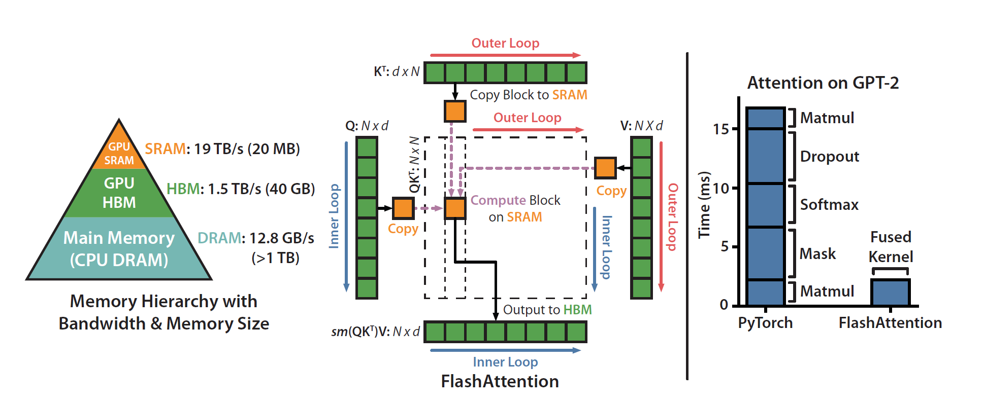
For training with typical batch sizes, attention memory can drop by 5-8×. Speedup varies but usually 2-3×.
The annoying part: Flash Attention can’t handle arbitrary attention masks. So for my sliding window attention in layers 1-8, I had to fall back to standard attention. Slower, but the window was small enough that it wasn’t terrible.
Two one-liners that made a surprising difference:
1 | torch.backends.cuda.matmul.allow_tf32 = True |
TF32 (TensorFloat-32) is NVIDIA’s format for matrix multiplications: fp32 range with reduced precision (10 bits instead of 23). It’s transparent, so you don’t change your code, just enable it. I measured a 15-20% speedup on H100 GPUs.
cuDNN benchmarking auto-tunes the convolution algorithms. Takes a few seconds at startup, but picks the fastest kernel for your specific shapes.
torch.compile
is maybe PyTorch 2.0’s best feature. JIT-compiles your model, fuses ops,
reduces kernel launches.
1 | model = torch.compile(model, mode='reduce-overhead', dynamic=True) |
mode='reduce-overhead' optimizes for fewer kernel
launches (takes longer to compile, but worth it).
dynamic=True handles variable batch sizes, which I needed
since I’m doing gradient accumulation.
Got about 20-30% speedup. First iteration is painfully slow while it compiles, and some ops don’t compile cleanly, but overall a solid win.
With 16 layers, activation memory adds up fast. Gradient checkpointing trades compute for memory: instead of storing all activations, recompute them during the backward pass.
1 | if self.gradient_checkpointing and (i % self.checkpoint_every == 0): |
I checkpoint every layer. Cuts activation memory by ~70%, lets me use bigger batches. The recompute overhead is maybe 20% slower per iteration, but worth it for the memory.
Optimizer Stuff
I tried Muon, which is getting some hype lately. It’s a second-order optimizer (like Shampoo but less annoying to implement). Uses preconditioned gradients instead of raw gradients. For 1D parameters (biases, layer norm scales), it falls back to AdamW.
1 | optimizer = MuonWithAuxAdam([ |
Not everything in the network should learn at the same speed:
- Embeddings: 2e-3 (highest, sparse updates can handle it)
- Layers 1-8: 8e-4 (local features, change fairly quickly)
- Layers 9-16: 6e-4 (global features, needs more stability)
- LM head: 4e-4 (lowest, go too high and logits explode)
These numbers came from trial and error. Early layers learn local patterns pretty easily, so they can move faster. Later layers do more abstract stuff and need to be more careful.
For the schedule, I used linear warmup for 1000 steps, then cosine decay down to 10% of peak LR. The formula is:
During warmup (\(t < t_{warmup}\)):
\[\eta(t) = \eta_{\max} \cdot \frac{t}{t_{\text{warmup}}}\]
After warmup (\(t \geq t_{warmup}\)):
\[\eta(t) = \eta_{\min} + \frac{1}{2}(\eta_{\max} - \eta_{\min}) \left(1 + \cos\left(\pi \frac{t - t_{\text{warmup}}}{t_{\text{total}} - t_{\text{warmup}}}\right)\right)\]
Warmup stops things from exploding early (random weights = crazy gradients). Cosine decay helps it converge at the end.
VRAM’s limited, so I couldn’t fit huge batches. The workaround: accumulate gradients over 2 micro-batches before stepping the optimizer. Effectively doubles batch size for free (memory-wise).
1 | for micro_step in range(2): |
Just remember to divide the loss by the accumulation steps so gradients stay scaled correctly.
How Training Went
Trained on Wikipedia + OpenWebText, about 10B tokens, 50k steps total.
Loss converged smoothly. No weird spikes, so the LR schedule and gradient clipping did their job.
The warmup’s visible in the first 1000 steps, then it’s all cosine decay. The different layer LRs stay proportional throughout.
Throughput climbed during the first few thousand steps while
torch.compile warmed up, then stabilized around 12k
tokens/sec.
Here’s how the U-Net gates evolved during training:
Layers 9-10 (early in the up-path) learned to rely more on skip connections (gates around 0.5-0.6). Layers 14-16 (near the output) kept their gates lower (0.1-0.25), suggesting they trust their own features more.
Stayed comfortably under the 80GB limit. Without gradient checkpointing and FP8, I’d be pushing 55-65GB and stuck with smaller batches.
What Actually Helped
After all this, what made a difference?
The U-Net skip connections gave maybe 5% better loss. Not huge, but the gates learned different values per layer instead of collapsing to the same thing, so I’m pretty sure the network was using them.
Mixed attention (MHA + MQA) didn’t speed up training much, but inference was about 15% faster because of the smaller KV cache.
Layerwise learning rates surprised me. Got around 8% better loss when I thought maybe 2-3% at best. The embedding layer really does want that higher LR.
FP8 attention was the big win. It gave 35% more throughput. Half the KV cache memory meant I could double batch size.
torch.compile is basically a free 25% speedup if you can deal with the first-iteration compile time.
Gradient checkpointing cut memory by 70%. Without it, I couldn’t fit the model at reasonable batch sizes. Slower iterations, but way more memory.
All of this let me train a ~300M parameter model on a single H100 in days instead of weeks. Not breaking any records, but good enough for experimenting.
Things That Flopped
Not everything worked:
Auxiliary loss at layer 8: Thought I’d add a second LM head at layer 8 to help the down-path learn better. Network just ignored it. The loss weight kept shrinking toward zero during training.
Bigger sliding windows: Tried 512 and 1024. No improvement, way slower. 256 was the sweet spot.
Fancy gate initializations: Tried 0.5, 0.0, even per-dimension learnable gates. Everything converged to about the same place. 0.1 worked fine.
Stochastic depth: Randomly dropping layers (DropPath style) didn’t help. Maybe works for really deep models, but at 16 layers it just hurt convergence.
Code
Full implementation is in my llm repo. Key files:
model/transformer.py: Hybrid U-Net Transformer architecturemodel/attention.py: MHA and MQA with FP8 supportmodel/ffn.py: Squared ReLU with learnable exponenttrain/loop.py: Training loop with all the optimizationstrain/optim.py: Muon optimizer and learning rate schedules
It’s not production-ready (no distributed training, no proper checkpointing, lots of rough edges), but it works for research.
What’s Next
Few things I want to try:
Scaling to 1B+ parameters. Does the U-Net thing still help at that scale? Would probably need pipeline parallelism to even fit it.
Better tokenization. I’m using basic BPE right now. The byte-level stuff looks interesting.
Mixture of Experts. Replace some FFNs with MoE layers, might help with the capacity/speed tradeoff.
Quantization-aware training. Train in FP8 from the start instead of quantizing afterward. Some papers claim it works better, but I haven’t tried it yet.
Closing thoughts
This was a good reminder that LLM architectures aren’t completely solved. Everyone’s doing the same basic Transformer thing because it works, but there’s room to borrow ideas from other domains. Some will flop, some won’t.
The performance stuff ended up mattering just as much as the
architecture. FP8 attention, torch.compile, and gradient
checkpointing are not exciting research-wise, but they made the
difference between weeks of training and days. I can’t ignore that.
If you’re doing LLM pre-training on limited compute: enable
torch.compile and mixed precision (easiest wins), use Flash
Attention and FP8 if your GPU supports it, trade speed for memory with
gradient checkpointing, and tune learning rates per layer. And try weird
architectural ideas. Worst case, you learn something.