For a long time I treated linear algebra as one of those courses you sit through, pass, and try to forget. Then I started doing machine learning seriously and realized the entire field is built on it. Every matrix multiplication, every gradient update, every embedding lookup is linear algebra in some form.
Vectors and matrices, everywhere
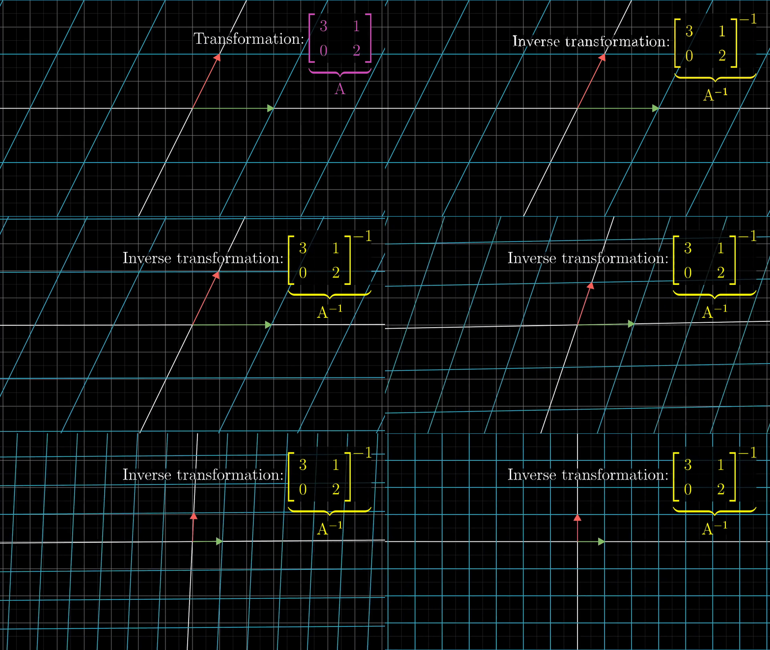
A dataset with \(n\) features lives in \(\mathbb{R}^n\). Each data point is a vector. When you apply a linear transformation, you multiply by a matrix \(A\):
\[f(x) = Ax\]
That one operation is the building block of every layer in a neural network. Stack a few of those, drop nonlinearities between them, and you have deep learning.
1 | import numpy as np |
I find it useful to remember that no matter how impressive a model architecture looks on paper, somewhere underneath it is still doing \(Wx + b\) in a loop.
Where it keeps showing up
PCA
Principal component analysis finds the directions in which your data varies the most. You compute the covariance matrix:
\[C = \frac{1}{n} X^T X\]
then solve the eigenvalue problem:
\[Cv = \lambda v\]
The eigenvectors with the largest eigenvalues point along the directions of largest variance. Project your data onto the top few of them and you get a lower-dimensional version that keeps most of the signal.
1 | def compute_pca(X: np.ndarray, n_components: int) -> tuple[np.ndarray, np.ndarray]: |
Neural network layers
Every layer of a neural network is a linear transformation followed by a nonlinearity:
\[h = \sigma(Wx + b)\]
The interesting part is in the weights. The transformation itself is the easy part.
1 | def neural_network_layer(X, W, b, activation): |
Gradient descent
Training is mostly subtracting matrices from each other:
\[W_{t+1} = W_{t} - \alpha \frac{\partial L}{\partial W_{t}}\]
The gradient \(\partial L / \partial W\) is itself a matrix the same shape as \(W\), and you update one with the other.
SVD
Singular value decomposition factorizes a matrix as:
\[A = U\Sigma V^T\]
I keep finding new places to use it, from low-rank approximations to recommendation systems to compressing model weights. Truncated SVD is the version I reach for most often, when I want to keep only the top \(k\) singular values:
1 | def truncated_svd(X: np.ndarray, k: int): |
Why the math view is worth keeping
When something breaks during training, having a feel for the underlying linear algebra makes debugging much faster. Loss exploding usually points at exponents or normalization. Gradients vanishing usually points at the eigenvalues of your weight matrices. A model that refuses to learn often turns out to have linearly dependent features and a rank-deficient matrix.
You can get pretty far without thinking about any of this. The moment things start going wrong, though, the math is what tells you where to look.