<?xml version="1.0" encoding="utf-8"?>
<feed xmlns="http://www.w3.org/2005/Atom">
  <title>dilawar.ai</title>
  <icon>https://www.dilawar.ai/icon.png</icon>
  
  <link href="https://www.dilawar.ai/atom.xml" rel="self"/>
  
  <link href="https://www.dilawar.ai/"/>
  <updated>2026-10-28T18:47:53.825Z</updated>
  <id>https://www.dilawar.ai/</id>
  
  <author>
    <name>Dilawar Mahmood</name>
    
  </author>
  
  <generator uri="https://hexo.io/">Hexo</generator>
  
  <entry>
    <title>Recurse Center Return Statement</title>
    <link href="https://www.dilawar.ai/2025/10/27/Recurse%20Center%20Return%20Statement/"/>
    <id>https://www.dilawar.ai/2025/10/27/Recurse%20Center%20Return%20Statement/</id>
    <published>2025-10-27T01:00:00.000Z</published>
    <updated>2026-10-28T18:47:53.825Z</updated>
    
    <content type="html"><![CDATA[<div style="display: flex; justify-content: center;"><p><img alt="Recurse Center logo: a pixel-art computer with a green face." src="https://d29xw0ra2h4o4u.cloudfront.net/assets/logo_square-60e12570c3a1b0b0798e651a0755f71a40ff15421761b786f720e4c02fc89a1f.png" style="max-width: 600px; width: 100%;"/></p></div><p>I’ve just finished three months at the <ahref="https://www.recurse.com/">Recurse Center</a> in the S2’25 batch.This is my return statement, the reflection that Recursers traditionallywrite at the end of their time there.</p><h2 id="what-even-is-the-recurse-center">What even is the RecurseCenter?</h2><p>RC is a self-directed programming retreat in NYC. There are noclasses or grades, and you choose what to work on. You can join remotelyor spend time at the Brooklyn space, where other programmers are workingon their own projects and are often happy to talk or pair.</p><p>A batch lasts 6 or 12 weeks. People might be writing an operatingsystem, learning functional programming, building a Game Boy emulator,or working through a theorem prover. Being around that range ofinterests was one of the things I enjoyed most.</p><p>I met quant traders, creative coders, engineers from large techcompanies, researchers, engineering directors, and high schoolers. Theyhad different reasons for being there, but a shared interest in spendingtime on programming.</p><p>RC’s <a href="https://www.recurse.com/social-rules">social rules</a>help make it easier to ask questions and work together:</p><ul><li><strong>No well-actually’s</strong>: don’t be pedantic when someonemakes a minor mistake.</li><li><strong>No feigned surprise</strong>: don’t act shocked when someonedoesn’t know something.</li><li><strong>No backseat driving</strong>: don’t interrupt pairprogrammers with drive-by suggestions.</li><li><strong>No subtle -isms</strong>: no racism, sexism, homophobia, ortransphobia, even subtle or “joking” versions.</li></ul><p>People followed these rules in everyday conversations. I could ask abasic question without having to explain why I didn’t already know theanswer, which made it much easier to learn from others.</p><p>The <ahref="https://www.recurse.com/self-directives">self-directives</a>describe how RC encourages people to approach their time:</p><ul><li><strong>Work at the edge of your abilities.</strong> Push yourselfpast what’s already comfortable.</li><li><strong>Build your volitional muscles.</strong> Work on what youactually want to work on, not what you “should.”</li><li><strong>Learn generously.</strong> Share what you know and helpothers.</li></ul><h2 id="why-i-joined">Why I joined</h2><p>I applied because I felt I was losing some of my confidence as aprogrammer. I wanted time to work on problems that stretched meagain.</p><p>During my last year or so at Apple, much of my time had gone intoproject management and coordinating work across teams. That work wasnecessary, but it left less room for the programming I wanted to do. Imissed spending long stretches working through a difficult technicalproblem.</p><p>I considered taking a vacation or finding more room for a sideproject at work. Then my mentor at Apple left for RC for similarreasons. Seeing someone I respected make that choice helped me decide toapply. Three months spent building things with other programmers soundedlike what I needed.</p><h2 id="what-i-worked-on">What I worked on</h2><p>I expected to spend time on lots of different topics. I did explore afew, but two projects ended up taking most of my attention.</p><p><strong>Distributed training on heterogeneous hardware.</strong> Iwanted to see whether I could train a model using different kinds ofaccelerators together. At RC, that meant finding a way for NVIDIA GPUsand my MacBook’s Apple Silicon to contribute to the same training run. Iwrote about the experiment <ahref="https://www.dilawar.ai/2025/07/04/Multi-Cluster%20Distributed%20Training%20on%20Heterogeneous%20Hardware/">here</a>.</p><p><strong>Alternative architectures for LLM pre-training.</strong> Inthe second half of the batch, I spent most of my time on language modelarchitectures and training performance under a limited compute budget. Ibuilt a hybrid U-Net Transformer and wrote up <ahref="https://www.dilawar.ai/2025/10/16/Pre-Training%20a%20Hybrid%20U-Net%20Transformer/">theexperiments</a>. A few researchers who are now at Anthropic helped methink through the design, and I’m grateful for their time.</p><p>Pairing also gave me a chance to work on things outside those twoprojects.</p><p><strong>Automatic theorem proving.</strong> An RC alum who hadrecently defended her PhD in geometric group theory worked through the<a href="https://github.com/leanprover-community/nng4">Natural NumberGame</a> with me in Lean. Congratulations again on the PhD! It was adifferent way of thinking about proofs from what I was used to.</p><p><strong>Other pairing sessions.</strong> These included a Game Boyemulator in C, figuring out when <ahref="https://en.wikipedia.org/wiki/Manhattanhenge">Manhattanhenge</a>happens, and several AI/ML applications. One person was building whatthey described as “Spotlight on steroids” for their localfilesystem.</p><p>I wish I’d paired more. Watching someone else work through a problemoften showed me an approach I wouldn’t have thought to try on myown.</p><h2 id="the-non-coding-parts">The non-coding parts</h2><p>Outside programming, I spent a lot of time playing chess, LoveLetter, and Decrypto. The game nights are some of my favorite memoriesof the batch, and many of my conversations with people happened overcards.</p><p>I also started <strong>Film Night</strong> in response to MovieNight. Movie Night had high-brow films and long discussions afterwards,so Film Night was for things that were fun and dumb. Our discussionswere more along the lines of “I liked the explosions” and “the maincharacter was hot.” I was quite happy with this contribution to RC’scultural life.</p><h2 id="what-i-got-out-of-it">What I got out of it</h2><p>I left RC feeling more confident in my programming and machinelearning work than I had in a long time. Having the time to follow aquestion through to an implementation made a real difference.</p><p>The facilitators helped me use the time well. Their advice gave meenough direction to keep making progress while leaving the choice ofprojects to me.</p><p>I also enjoyed programming in a way I hadn’t for a while. I couldspend a day understanding something difficult, ask someone nearby forhelp, and see where the conversation led. That was the kind of work I’dbeen missing when I applied.</p><p>If that sounds appealing, <ahref="https://www.recurse.com/apply">take a look at RC</a>. I’m glad Imade time for it, both for the projects and for the people I met.</p><p>Never graduate! 🌱</p>]]></content>


    <summary type="html">&lt;div style=&quot;display: flex; justify-content: center;&quot;&gt;
&lt;p&gt;&lt;img alt=&quot;Recurse Center logo: a pixel-art computer with a green face.&quot;</summary>


    <category term="Recurse Center" scheme="https://www.dilawar.ai/tags/Recurse-Center/"/>
    
  </entry>
  
  <entry>
    <title>Pre-Training a Hybrid U-Net Transformer</title>
    <link href="https://www.dilawar.ai/2025/10/16/Pre-Training%20a%20Hybrid%20U-Net%20Transformer/"/>
    <id>https://www.dilawar.ai/2025/10/16/Pre-Training%20a%20Hybrid%20U-Net%20Transformer/</id>
    <published>2025-10-16T14:30:00.000Z</published>
    <updated>2026-10-28T18:47:53.825Z</updated>
    
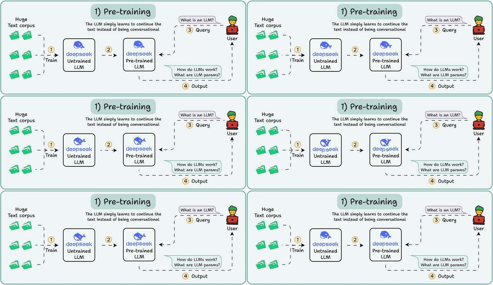
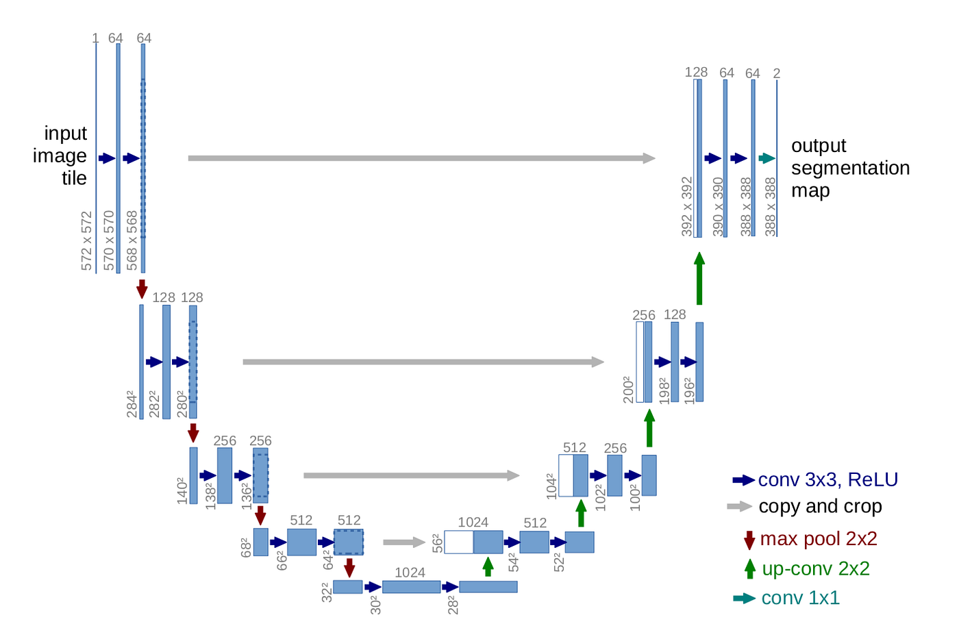
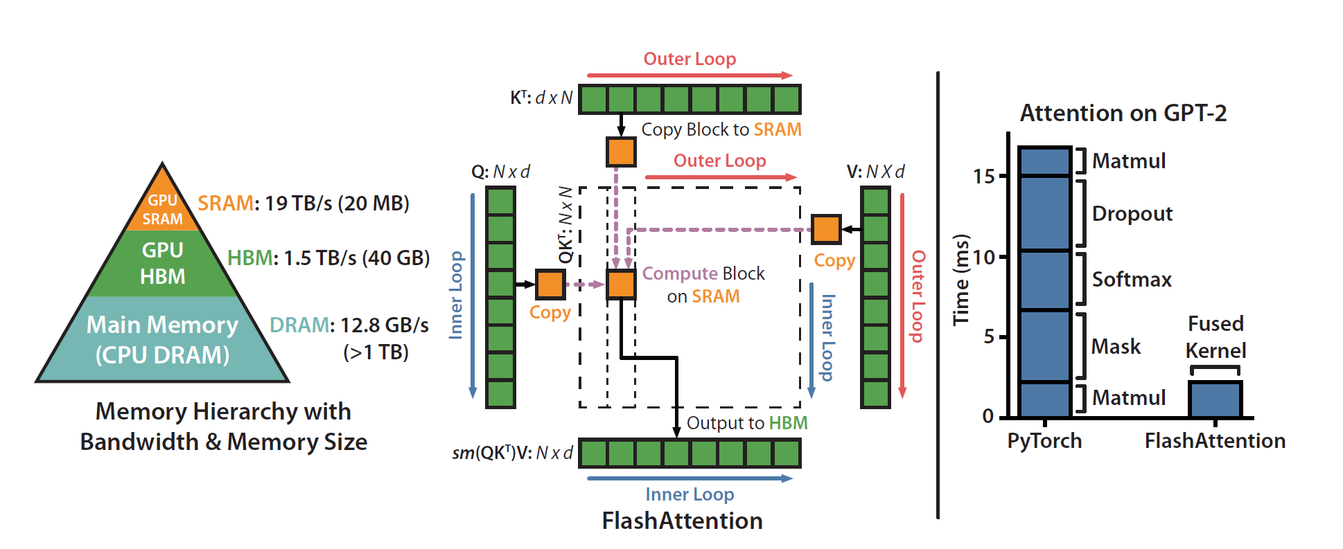
    <content type="html"><![CDATA[<div style="display: flex; justify-content: center;"><p><img alt="Language model pre-training on a large text corpus, followed by a user query and model output." src="https://substackcdn.com/image/fetch/$s_!H24w!,f_auto,q_auto:good,fl_progressive:steep/https%3A%2F%2Fsubstack-post-media.s3.amazonaws.com%2Fpublic%2Fimages%2F7c2b8c79-de81-4c65-9f81-96277f53de25_1474x568.gif" style="max-width: 600px; width: 100%;"/></p></div><p>During my batch at the Recurse Center, I’ve been experimenting withlanguage model pre-training on a limited compute budget. I wanted to trychanges to the Transformer architecture while also working on thetraining code, since faster runs would give me more room to compareideas.</p><p>I spent most of that time on skip connections inspired by U-Net,using them to combine representations from earlier and later Transformerlayers.</p><h2 id="why-u-net">Why U-Net?</h2><p>U-Net was <a href="https://arxiv.org/abs/1505.04597">introduced forbiomedical image segmentation</a>. Its encoder reduces spatialresolution as it builds features, and its decoder combines thosefeatures with earlier ones through skip connections. That lets theoutput use both local detail and information gathered at lowerresolutions.</p><p>I wanted to test a similar connection pattern in a language model. Myversion keeps the sequence length fixed and pairs layers by depth, so itborrows U-Net’s skip structure without reproducing its spatialdownsampling and upsampling.</p><div style="display: flex; justify-content: center;"><p><img alt="U-Net encoder and decoder connected by skip connections at corresponding resolutions." src="https://miro.medium.com/v2/resize:fit:1400/1*f7YOaE4TWubwaFF7Z1fzNw.png" style="max-width: 600px; width: 100%;"/></p></div><p>I split 16 Transformer layers into two groups. Layers 1 through 8save their activations, and layers 9 through 16 combine them with theirown activations through learned gates.</p><p>Each gate has one learned parameter per hidden dimension, initializedto 0.1. It combines the two inputs as follows:</p><p><span class="math display">\[\text{output} = \text{gate} \times\text{skip} + (1 - \text{gate}) \times \text{current}\]</span></p><p>A larger gate gives the saved activation more weight, while a smallergate gives the current activation more weight. Because each layer hasits own gate, training can adjust these contributions separately.</p><p>The mixing module is small:</p><figure tabindex="0" role="region" aria-label="Code example 1" data-scroll-region class="highlight python"><table role="presentation"><tr><td class="gutter" aria-hidden="true"><pre><span class="line">1</span><br><span class="line">2</span><br><span class="line">3</span><br><span class="line">4</span><br><span class="line">5</span><br><span class="line">6</span><br><span class="line">7</span><br></pre></td><td class="code"><pre><span class="line"><span class="keyword">class</span> <span class="title class_">GatedMixer</span>(nn.Module):</span><br><span class="line">    <span class="keyword">def</span> <span class="title function_">__init__</span>(<span class="params">self, d_model: <span class="built_in">int</span></span>) -&gt; <span class="literal">None</span>:</span><br><span class="line">        <span class="built_in">super</span>().__init__()</span><br><span class="line">        <span class="variable language_">self</span>.gate = nn.Parameter(torch.full((<span class="number">1</span>, <span class="number">1</span>, d_model), <span class="number">0.1</span>))</span><br><span class="line"></span><br><span class="line">    <span class="keyword">def</span> <span class="title function_">forward</span>(<span class="params">self, skip: torch.Tensor, current: torch.Tensor</span>) -&gt; torch.Tensor:</span><br><span class="line">        <span class="keyword">return</span> <span class="variable language_">self</span>.gate * skip + (<span class="number">1</span> - <span class="variable language_">self</span>.gate) * current</span><br></pre></td></tr></table></figure><p>The saved activations are used in reverse order: layer 9 receiveslayer 8’s output, layer 10 receives layer 7’s, and so on. This createsconnections between matching positions in the two halves of themodel.</p><h2 id="not-all-layers-are-equal">Not all layers are equal</h2><p>I also split the attention mechanisms between the two halves. Theidea was to let the earlier layers work with nearby tokens, then givethe later layers access to the full preceding context.</p><p>Layers 1 through 8 use sliding-window <ahref="https://arxiv.org/abs/1706.03762">multi-head attention</a>,following the local-attention idea used in <ahref="https://arxiv.org/abs/2004.05150">Longformer</a>. Each query islimited to a window ending at its own position, which preserves thecausal constraint.</p><div style="display: flex; justify-content: center;"><p><img alt="Attention patterns: full attention, sliding windows, dilated sliding windows, and global plus sliding-window attention." src="https://media.geeksforgeeks.org/wp-content/uploads/20231108170402/Longformer-attention-Mechanism-file.png" style="max-width: 600px; width: 100%;"/></p></div><p>In the window described here, position <spanclass="math inline">\(i\)</span> can attend to positions in <spanclass="math inline">\([i - 256, i]\)</span>. These layers don’t directlyattend to distant tokens; the upper layers provide the widercontext.</p><p>Layers 9 through 16 use <ahref="https://arxiv.org/abs/1911.02150">multi-query attention (MQA)</a>.The query heads share key and value projections, reducing the amount ofkey and value data that needs to be stored during autoregressiveinference.</p><div style="display: flex; justify-content: center;"><p><img alt="Multi-head, grouped-query, and multi-query attention compared by how queries share keys and values." src="https://miro.medium.com/v2/resize:fit:1052/1*NI-Bq7my9w99Px-d6WTKmA.png" style="max-width: 600px; width: 100%;"/></p></div><p>With 8 heads and <code>d_model=1024</code>, each head has 128dimensions. Standard multi-head attention stores a separate key andvalue for each head, while MQA shares one pair across all eight. At thesame sequence length, the MQA layer therefore uses about one eighth asmuch KV cache storage.</p><p>Both attention types use <ahref="https://arxiv.org/abs/2104.09864">RoPE</a> to represent position.RoPE rotates query and key vectors according to their positions, sotheir dot product also depends on the relative distance betweenthem.</p><div style="display: flex; justify-content: center;"><p><img alt="Rotary position encoding rotates query and key vectors in the complex plane." src="https://media.licdn.com/dms/image/v2/D5612AQHEc_1lzl2c6w/article-cover_image-shrink_600_2000/article-cover_image-shrink_600_2000/0/1729397421043?e=2147483647&v=beta&t=lALiM_f2DyUGVyHUV5SuLBJuAP5Dccx8zexecW5iGII" style="max-width: 600px; width: 100%;"/></p></div><p>The rotation is computed using sine and cosine functions:</p><p><span class="math display">\[\text{freq}_{j} =\frac{1}{10000^{2j/d}}\]</span></p><p><span class="math display">\[\text{RoPE}(x, \text{pos}) =\begin{pmatrix} x_{1} \\ x_{2} \\ \vdots \end{pmatrix} \odot\begin{pmatrix} \cos(\text{pos} \cdot \text{freq}) \\ \cos(\text{pos}\cdot \text{freq}) \\ \vdots \end{pmatrix} + \text{rotate\_half}(x)\odot \begin{pmatrix} \sin(\text{pos} \cdot \text{freq}) \\\sin(\text{pos} \cdot \text{freq}) \\ \vdots \end{pmatrix}\]</span></p><p>The rotation can be calculated beyond the sequence lengths used intraining, but that doesn’t guarantee the model will work well at thoselengths. I would still need to evaluate longer-context inferenceseparately.</p><h2 id="letting-activation-functions-learn">Letting activation functionslearn</h2><p>The feedforward blocks start with squared ReLU, <spanclass="math inline">\(\text{ReLU}(x)^2\)</span>. The <ahref="https://arxiv.org/abs/2109.08668">Primer paper</a> includes thischange among the modifications that improved its language models. Iwanted to see what would happen if the exponent could vary by layer.</p><p>I initialized a learned exponent at 2 and allowed training to adjustit:</p><figure tabindex="0" role="region" aria-label="Code example 2" data-scroll-region class="highlight python"><table role="presentation"><tr><td class="gutter" aria-hidden="true"><pre><span class="line">1</span><br><span class="line">2</span><br><span class="line">3</span><br><span class="line">4</span><br><span class="line">5</span><br><span class="line">6</span><br><span class="line">7</span><br><span class="line">8</span><br><span class="line">9</span><br><span class="line">10</span><br><span class="line">11</span><br><span class="line">12</span><br><span class="line">13</span><br><span class="line">14</span><br><span class="line">15</span><br></pre></td><td class="code"><pre><span class="line"><span class="keyword">class</span> <span class="title class_">SquaredReLUFFN</span>(nn.Module):</span><br><span class="line">    <span class="keyword">def</span> <span class="title function_">__init__</span>(<span class="params">self, d_model: <span class="built_in">int</span>, expansion: <span class="built_in">float</span></span>) -&gt; <span class="literal">None</span>:</span><br><span class="line">        <span class="built_in">super</span>().__init__()</span><br><span class="line">        hidden = <span class="built_in">int</span>(d_model * expansion)</span><br><span class="line">        <span class="variable language_">self</span>.w1 = nn.Linear(d_model, hidden)</span><br><span class="line">        <span class="variable language_">self</span>.w2 = nn.Linear(hidden, d_model)</span><br><span class="line">        <span class="variable language_">self</span>.alpha = nn.Parameter(torch.tensor(<span class="number">2.0</span>))  <span class="comment"># learnable exponent</span></span><br><span class="line"></span><br><span class="line">    <span class="keyword">def</span> <span class="title function_">forward</span>(<span class="params">self, x: torch.Tensor</span>) -&gt; torch.Tensor:</span><br><span class="line">        x = <span class="variable language_">self</span>.w1(x)</span><br><span class="line">        x = torch.relu(x)</span><br><span class="line">        alpha = torch.clamp(<span class="variable language_">self</span>.alpha, <span class="number">0.5</span>, <span class="number">4.0</span>)  <span class="comment"># keep it reasonable</span></span><br><span class="line">        x = torch.<span class="built_in">pow</span>(x + <span class="number">1e-6</span>, alpha)</span><br><span class="line">        x = <span class="variable language_">self</span>.w2(x)</span><br><span class="line">        <span class="keyword">return</span> x</span><br></pre></td></tr></table></figure><p>Some layers settled near <span class="math inline">\(\alpha \approx2.3\)</span>, while others stayed around 2.0 or moved toward 1.8. Thatshowed the parameter was changing during training, although comparingagainst a fixed-exponent model is still necessary to tell whether ithelps the final result.</p><p>I also varied the FFN expansion ratio by layer:</p><ul><li>Layers 1-8: 4× expansion (4096 hidden for<code>d_model=1024</code>).</li><li>Layers 9-16: 2.5× expansion (2560 hidden).</li></ul><p>This gives the lower half more feedforward capacity while keeping theupper half smaller. It was a design choice to test alongside theattention split, rather than something I knew would be better inadvance.</p><h2 id="making-it-actually-run">Making it actually run</h2><p>A 16-layer model with a hidden size of 1024 was large enough thattraining time and memory use constrained the experiments. I workedthrough several optimizations to make repeated runs practical.</p><p>I started with <ahref="https://pytorch.org/docs/stable/amp.html">bfloat16 mixedprecision</a>. Autocast runs eligible operations at lower precisionwhile other operations and the parameter gradients can remain infp32:</p><figure tabindex="0" role="region" aria-label="Code example 3" data-scroll-region class="highlight python"><table role="presentation"><tr><td class="gutter" aria-hidden="true"><pre><span class="line">1</span><br><span class="line">2</span><br><span class="line">3</span><br><span class="line">4</span><br></pre></td><td class="code"><pre><span class="line"><span class="keyword">with</span> torch.amp.autocast(device_type=<span class="string">&#x27;cuda&#x27;</span>, dtype=torch.bfloat16):</span><br><span class="line">    logits = model(input_ids)</span><br><span class="line">    loss = cross_entropy(logits, targets)</span><br><span class="line">loss.backward()</span><br></pre></td></tr></table></figure><p>Bfloat16 has the same 8-bit exponent range as fp32, with 7 bits offraction precision instead of 23. That wider range was useful foravoiding some overflow problems associated with fp16. It still losesprecision, so the loss and gradients needed checking duringtraining.</p><p>I also used NVIDIA’s <ahref="https://github.com/NVIDIA/TransformerEngine">TransformerEngine</a> to run supported attention operations in FP8. A value storedin FP8 takes half the space of bf16, although the memory savings for thewhole model depend on which tensors use it. In these experiments, theFP8 setup gave roughly 30 to 40% more throughput and allowed largerbatches:</p><figure tabindex="0" role="region" aria-label="Code example 4" data-scroll-region class="highlight python"><table role="presentation"><tr><td class="gutter" aria-hidden="true"><pre><span class="line">1</span><br><span class="line">2</span><br><span class="line">3</span><br><span class="line">4</span><br></pre></td><td class="code"><pre><span class="line"><span class="keyword">if</span> <span class="variable language_">self</span>.use_fp8 <span class="keyword">and</span> te <span class="keyword">is</span> <span class="keyword">not</span> <span class="literal">None</span>:</span><br><span class="line">    hidden_states = x.transpose(<span class="number">0</span>, <span class="number">1</span>).contiguous()</span><br><span class="line">    <span class="keyword">with</span> te.fp8_autocast(enabled=<span class="literal">True</span>):</span><br><span class="line">        output = <span class="variable language_">self</span>._te_mha(hidden_states)</span><br></pre></td></tr></table></figure><p>Those results came from an H100. The available FP8 kernels depend onthe GPU and the Transformer Engine version, so the same setup needschecking before moving it to other hardware.</p><p><a href="https://arxiv.org/abs/2205.14135">FlashAttention</a> reducesattention’s memory traffic by calculating it in blocks without storingthe full attention matrix. PyTorch’s<code>scaled_dot_product_attention</code> can select a fusedimplementation when the inputs and hardware support it:</p><div style="display: flex; justify-content: center;"><p><img alt="FlashAttention uses GPU memory tiling to reduce memory transfers and attention computation time." src="https://miro.medium.com/v2/resize:fit:2000/1*i4tDdwgvGtXuTIyJpFUn8A.png" style="max-width: 600px; width: 100%;"/></p></div><p>For the batch sizes I tested, attention memory use fell by 5 to 8×and end-to-end training was roughly 2 to 3× faster.</p><p>The sliding-window mask in my implementation didn’t use the same fastpath, so layers 1 through 8 fell back to standard attention. Thatlimited the speedup, even with the smaller attention window.</p><p>I also enabled these backend settings:</p><figure tabindex="0" role="region" aria-label="Code example 5" data-scroll-region class="highlight python"><table role="presentation"><tr><td class="gutter" aria-hidden="true"><pre><span class="line">1</span><br><span class="line">2</span><br></pre></td><td class="code"><pre><span class="line">torch.backends.cuda.matmul.allow_tf32 = <span class="literal">True</span></span><br><span class="line">torch.backends.cudnn.benchmark = <span class="literal">True</span></span><br></pre></td></tr></table></figure><p><ahref="https://blogs.nvidia.com/blog/tensorfloat-32-precision-format/">TF32(TensorFloat-32)</a> lets supported matrix multiplications use reducedmantissa precision while retaining fp32’s exponent range. I measured a15 to 20% speedup in my H100 tests. The setting affects eligible fp32operations, so its contribution depends on how much of the workloadalready runs in bf16 or FP8.</p><p>cuDNN benchmarking searches for a suitable convolution algorithm forthe input shapes. It only matters where the model uses convolutionoperations; it doesn’t accelerate the attention layers themselves.</p><p><ahref="https://pytorch.org/tutorials/intermediate/torch_compile_tutorial.html"><code>torch.compile</code></a>captures parts of the model for compilation and can fuse operations toreduce overhead:</p><figure tabindex="0" role="region" aria-label="Code example 6" data-scroll-region class="highlight python"><table role="presentation"><tr><td class="gutter" aria-hidden="true"><pre><span class="line">1</span><br></pre></td><td class="code"><pre><span class="line">model = torch.<span class="built_in">compile</span>(model, mode=<span class="string">&#x27;reduce-overhead&#x27;</span>, dynamic=<span class="literal">True</span>)</span><br></pre></td></tr></table></figure><p>The <code>reduce-overhead</code> mode uses CUDA graphs whereapplicable to reduce Python overhead, while <code>dynamic=True</code>asks the compiler to handle changing shapes. Compilation made the firstiteration slow, and some operations needed extra work to compile, butsteady-state throughput improved by about 20 to 30%.</p><p><a href="https://pytorch.org/docs/stable/checkpoint.html">Gradientcheckpointing</a> reduced the activations I needed to keep in memory. Itrecomputes them during the backward pass:</p><figure tabindex="0" role="region" aria-label="Code example 7" data-scroll-region class="highlight python"><table role="presentation"><tr><td class="gutter" aria-hidden="true"><pre><span class="line">1</span><br><span class="line">2</span><br><span class="line">3</span><br><span class="line">4</span><br></pre></td><td class="code"><pre><span class="line"><span class="keyword">if</span> <span class="variable language_">self</span>.gradient_checkpointing <span class="keyword">and</span> (i % <span class="variable language_">self</span>.checkpoint_every == <span class="number">0</span>):</span><br><span class="line">    h = checkpoint(<span class="keyword">lambda</span> inp: <span class="variable language_">self</span>.blocks[i](inp, attn_mask), h, use_reentrant=<span class="literal">False</span>)</span><br><span class="line"><span class="keyword">else</span>:</span><br><span class="line">    h = <span class="variable language_">self</span>.blocks[i](h, attn_mask)</span><br></pre></td></tr></table></figure><p>Checkpointing every layer reduced activation memory by roughly 70%.Iterations took about 20% longer, but the extra memory allowed largerbatches, which made the trade worthwhile for this setup.</p><h2 id="optimizer-choices">Optimizer choices</h2><p>I tried <a href="https://github.com/KellerJordan/modded-nanogpt">Muonin modded-nanogpt</a>, which applies an orthogonalization step tomomentum-based updates for matrix weights. The <ahref="https://kellerjordan.github.io/posts/muon/">optimizer’sdescription</a> explains that step and which parameters should use aconventional optimizer. I used an AdamW group for the parameters outsidethe Muon group:</p><figure tabindex="0" role="region" aria-label="Code example 8" data-scroll-region class="highlight python"><table role="presentation"><tr><td class="gutter" aria-hidden="true"><pre><span class="line">1</span><br><span class="line">2</span><br><span class="line">3</span><br><span class="line">4</span><br></pre></td><td class="code"><pre><span class="line">optimizer = MuonWithAuxAdam([</span><br><span class="line">    &#123;<span class="string">&quot;params&quot;</span>: muon_params, <span class="string">&quot;lr&quot;</span>: <span class="number">8e-4</span>, <span class="string">&quot;use_muon&quot;</span>: <span class="literal">True</span>&#125;,</span><br><span class="line">    &#123;<span class="string">&quot;params&quot;</span>: adamw_params, <span class="string">&quot;lr&quot;</span>: <span class="number">8e-4</span>, <span class="string">&quot;betas&quot;</span>: (<span class="number">0.9</span>, <span class="number">0.95</span>)&#125;</span><br><span class="line">])</span><br></pre></td></tr></table></figure><p>I used different peak learning rates for different parts of themodel:</p><ul><li>Embeddings: 2e-3.</li><li>Layers 1-8: 8e-4.</li><li>Layers 9-16: 6e-4.</li><li>LM head: 4e-4.</li></ul><p>These settings came from trial and error. Higher rates worked betterfor the embeddings in these runs, while the upper layers and output headwere more stable with smaller updates.</p><p>The schedule used 1,000 warmup steps followed by cosine decay to 10%of each group’s peak learning rate:</p><p>During warmup (<span class="math inline">\(t &lt;t_{\text{warmup}}\)</span>):</p><p><span class="math display">\[\eta(t) = \eta_{\max} \cdot\frac{t}{t_{\text{warmup}}}\]</span></p><p>After warmup (<span class="math inline">\(t \geqt_{\text{warmup}}\)</span>):</p><p><span class="math display">\[\eta(t) = \eta_{\min} +\frac{1}{2}(\eta_{\max} - \eta_{\min}) \left(1 + \cos\left(\pi \frac{t -t_{\text{warmup}}}{t_{\text{total}} -t_{\text{warmup}}}\right)\right)\]</span></p><p>Warmup increases the step size gradually at the start of training.Cosine decay then reduces it as training progresses, allowing smallerupdates toward the end.</p><p>To increase the effective batch size without keeping all itsactivations in memory at once, I accumulated gradients over twomicro-batches before updating the weights:</p><figure tabindex="0" role="region" aria-label="Code example 9" data-scroll-region class="highlight python"><table role="presentation"><tr><td class="gutter" aria-hidden="true"><pre><span class="line">1</span><br><span class="line">2</span><br><span class="line">3</span><br><span class="line">4</span><br><span class="line">5</span><br></pre></td><td class="code"><pre><span class="line"><span class="keyword">for</span> micro_step <span class="keyword">in</span> <span class="built_in">range</span>(<span class="number">2</span>):</span><br><span class="line">    loss = forward_and_loss(batch) / <span class="number">2</span>  <span class="comment"># scale the loss</span></span><br><span class="line">    loss.backward()</span><br><span class="line">optimizer.step()</span><br><span class="line">optimizer.zero_grad()</span><br></pre></td></tr></table></figure><p>Dividing each loss by the number of accumulation steps keeps theaccumulated gradient on the intended scale.</p><h2 id="how-training-went">How training went</h2><p>I trained on Wikipedia and OpenWebText, using about 10B tokens over50,000 steps.</p><p><strong>About the plots:</strong> these charts are illustrationsgenerated by the page, rather than exported training logs. Thelearning-rate chart shows the configured schedule; the loss, throughput,gate, and memory charts use generated values.</p><figure class="article-chart" aria-label="Training and Validation Loss"><figcaption class="chart-title">Training and Validation Loss</figcaption><div id="loss-plot" class="chart-canvas" hidden=""></div><p class="chart-status" role="status">Interactive chart: Training and Validation Loss. Enable JavaScript toexplore it; the description below explains the illustration.</p><button class="chart-retry" type="button" hidden>Try chart again</button></figure><p>This illustration shows training and validation loss decreasingtogether, with a small gap between the two curves.</p><figure class="article-chart" aria-label="Layer-wise Learning Rate Schedules"><figcaption class="chart-title">Layer-wise Learning Rate Schedules</figcaption><div id="lr-plot" class="chart-canvas" hidden=""></div><p class="chart-status" role="status">Interactive chart: Layer-wise Learning Rate Schedules. Enable JavaScriptto explore it; the description below explains the illustration.</p><button class="chart-retry" type="button" hidden>Try chart again</button></figure><p>The learning-rate plot follows the schedule in the code: 1,000 stepsof warmup, followed by cosine decay. The rates for the differentparameter groups remain proportional throughout.</p><figure class="article-chart" aria-label="Training Throughput"><figcaption class="chart-title">Training Throughput</figcaption><div id="throughput-plot" class="chart-canvas" hidden=""></div><p class="chart-status" role="status">Interactive chart: Training Throughput. Enable JavaScript to explore it;the description below explains the illustration.</p><button class="chart-retry" type="button" hidden>Try chart again</button></figure><p>The throughput illustration shows an initial increase followed by asteady rate of around 12k tokens per second.</p><p>The next illustration shows how different layers could settle ondifferent gate values:</p><figure class="article-chart" aria-label="U-Net Gate Values During Training"><figcaption class="chart-title">U-Net Gate Values During Training</figcaption><div id="gates-plot" class="chart-canvas" hidden=""></div><p class="chart-status" role="status">Interactive chart: U-Net Gate Values During Training. Enable JavaScriptto explore it; the description below explains the illustration.</p><button class="chart-retry" type="button" hidden>Try chart again</button></figure><p>In this illustration, layers 9 and 10 have gates around 0.5 to 0.6,while layers 14 through 16 have values around 0.1 to 0.25. Higher gatevalues give more weight to the saved activations.</p><figure class="article-chart" aria-label="GPU Memory Usage (H100 80GB)"><figcaption class="chart-title">GPU Memory Usage (H100 80GB)</figcaption><div id="memory-plot" class="chart-canvas" hidden=""></div><p class="chart-status" role="status">Interactive chart: GPU Memory Usage (H100 80GB). Enable JavaScript toexplore it; the description below explains the illustration.</p><button class="chart-retry" type="button" hidden>Try chart again</button></figure><p>The memory illustration separates allocated from reserved memory andmarks the H100’s 80GB capacity. The batch size, precision, andcheckpointing settings all affect how much memory a run needs.</p><h2 id="what-actually-helped">What actually helped</h2><p>In my comparisons, the changes had the following effects. Theseresults are specific to this model and training setup.</p><p>The U-Net skip connections improved loss by roughly 5% in mycomparisons. The gate values differed across layers, which was useful toinspect, but their variation alone doesn’t explain the lossimprovement.</p><p>Combining MHA in the lower half with MQA in the upper half changedtraining speed little. Inference was about 15% faster, with the smallerKV cache in the MQA layers helping reduce the amount of datainvolved.</p><p>Using different learning rates by layer gave an improvement of around8% in the comparison, more than the 2 to 3% I had expected. The higherembedding rate accounted for an important part of that result.</p><p>The FP8 attention setup increased throughput by about 35%, and thereduced memory use allowed me to double the batch size.</p><p>After compilation, <code>torch.compile</code> gave roughly a 25%speedup. That was useful over a long run, despite the initialcompilation cost.</p><p>Checkpointing’s 70% reduction in activation memory was also usefuldespite the slower iterations. It let me use a reasonable batch sizewithout exceeding the GPU’s memory.</p><p>With these changes, I could train the 300M-parameter model on asingle H100 over a few days, which was enough to make furtherexperiments practical.</p><h2 id="things-that-flopped">Things that flopped</h2><p>Several other changes added complexity without improving theresult.</p><p><strong>Auxiliary loss at layer 8.</strong> I added a secondlanguage-model head halfway through the network and trained it on thesame targets. Its learned loss weight shrank toward zero, so itcontributed little to the final training objective.</p><p><strong>Bigger sliding windows.</strong> Increasing the window to 512or 1024 made training slower without improving loss in these runs, so Ikept the 256-token setting.</p><p><strong>Gate initialization.</strong> I tried starting the gates at0.5 and 0.0 as well as 0.1. The results were similar enough that I kept0.1.</p><p><strong>Stochastic depth.</strong> Randomly dropping layers,following the <a href="https://arxiv.org/abs/1605.07648">stochasticdepth idea</a>, hurt convergence in this 16-layer model.</p><h2 id="code">Code</h2><p>The implementation is in my <ahref="https://github.com/dilawarm/llm">llm repository</a>. The mainfiles are:</p><ul><li><ahref="https://github.com/dilawarm/llm/blob/main/llm/model/transformer.py"><code>model/transformer.py</code></a>:Hybrid U-Net Transformer architecture.</li><li><ahref="https://github.com/dilawarm/llm/blob/main/llm/model/attention.py"><code>model/attention.py</code></a>:MHA and MQA with FP8 support.</li><li><ahref="https://github.com/dilawarm/llm/blob/main/llm/model/ffn.py"><code>model/ffn.py</code></a>:Squared ReLU with learnable exponent.</li><li><ahref="https://github.com/dilawarm/llm/blob/main/llm/train/loop.py"><code>train/loop.py</code></a>:Training loop with all the optimizations.</li><li><ahref="https://github.com/dilawarm/llm/blob/main/llm/train/optim.py"><code>train/optim.py</code></a>:Muon optimizer and learning rate schedules.</li></ul><p>This is experimental code. It still lacks distributed training and acomplete checkpointing system, and some parts need more testing beforeI’d use them for a long unattended run.</p><h2 id="whats-next">What’s next</h2><p>I’d like to test whether the changes that helped here still help asthe model grows.</p><p>A model above 1B parameters would give me a useful next comparisonfor the U-Net connections. Depending on the batch size and memoryrequirements, I may also need to explore tensor or pipelineparallelism.</p><p>I also want to compare tokenizers. The current model uses basic BPE;<a href="https://github.com/openai/tiktoken">tiktoken’s byte-levelBPE</a> is one implementation to examine. I’d want to compare sequencelengths and downstream results before changing the training setup.</p><p><a href="https://arxiv.org/abs/2101.03961">Mixture of experts</a> isanother possibility. Replacing some feedforward blocks with expertlayers could add capacity without activating all of it for every token,though it would also add routing and training complexity.</p><p>I’d also like to extend low-precision training beyond the attentionpath used here. Work such as <ahref="https://arxiv.org/abs/2310.18313">FP8-LM</a> explores using FP8more broadly during training. I haven’t tested that approach yet.</p><h2 id="closing-thoughts">Making room for more experiments</h2><p>The U-Net connections gave me an architectural idea that I could testwithout building a completely different model. Some variations helped inthese experiments and others didn’t, so I want to keep comparing themagainst a plain Transformer as the setup changes.</p><p>Training speed mattered because it determined how many comparisons Icould afford to run. Mixed precision, compilation, and checkpointingmade the architectural experiments easier to carry out on the hardware Ihad.</p><p>For this project, it made sense to get a stable baseline and measurethe runtime changes before spending more time on architecturalvariations. That gave me a better chance of telling whether a resultcame from the model itself, the training settings, or theimplementation.</p><p><a href="https://github.com/dilawarm/llm">Code is on GitHub</a>.</p>]]></content>


    <summary type="html">&lt;div style=&quot;display: flex; justify-content: center;&quot;&gt;
&lt;p&gt;&lt;img alt=&quot;Language model pre-training on a large text corpus, followed by a user</summary>


    <category term="Machine Learning" scheme="https://www.dilawar.ai/tags/Machine-Learning/"/>
    
    <category term="LLM" scheme="https://www.dilawar.ai/tags/LLM/"/>
    
    <category term="Recurse Center" scheme="https://www.dilawar.ai/tags/Recurse-Center/"/>
    
    <category term="Performance Engineering" scheme="https://www.dilawar.ai/tags/Performance-Engineering/"/>
    
  </entry>
  
  <entry>
    <title>Being GPU Poor makes you creative</title>
    <link href="https://www.dilawar.ai/2025/07/04/Multi-Cluster%20Distributed%20Training%20on%20Heterogeneous%20Hardware/"/>
    <id>https://www.dilawar.ai/2025/07/04/Multi-Cluster%20Distributed%20Training%20on%20Heterogeneous%20Hardware/</id>
    <published>2025-07-04T21:24:00.000Z</published>
    <updated>2026-10-28T18:47:53.825Z</updated>
    
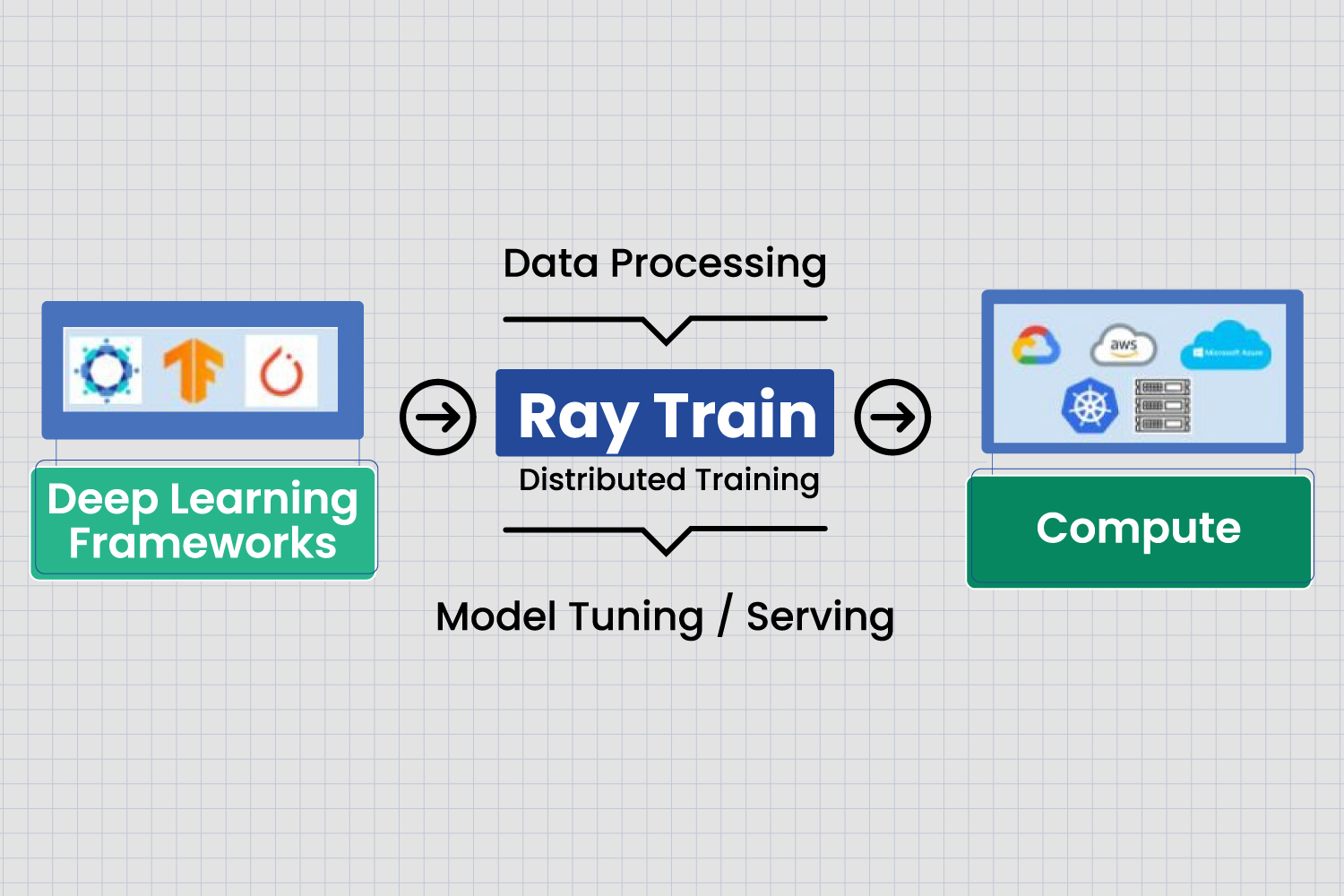
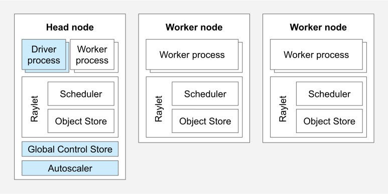
    <content type="html"><![CDATA[<div style="display: flex; justify-content: center;"><p><img alt="A black cap embroidered with “gpu poor.”" src="/images/gpu_poor.jpg" style="max-width: 600px; width: 100%;"/></p></div><p>At the start of my sabbatical, I went from having access to computeat Apple to working on my MacBook. On my first visit to the RecurseCenter hub in NYC, someone mentioned that there were a couple of GPUsavailable. I wanted to see whether I could put them to use alongside thelaptop.</p><p>The machines didn’t have much in common. RC had two NVIDIA GeForceGTX TITAN X cards, while my M4 Max MacBook used Apple Silicon. Theyneeded different runtimes and had different memory limits, so I needed away to coordinate training without assuming every worker had the samehardware.</p><p><a href="https://ray.io">Ray</a> came to mind because its actor modellooked like a reasonable way to coordinate the workers.</p><h2 id="the-heterogeneous-hardware-problem">The heterogeneous hardwareproblem</h2><p>A mixed set of machines is a fairly ordinary situation when you’reusing hardware that is already available. For this experiment, I had twokinds of workers:</p><ul><li><strong>MacBook M4 Max</strong>, Apple Silicon with MPS (MetalPerformance Shaders).</li><li><strong>RC machines</strong>, NVIDIA GeForce GTX TITAN X with CUDA.There were two of them, named Mercer and Crosby, because RC names itsmachines.</li></ul><p>A training setup built around CUDA and NCCL doesn’t directly includean MPS worker. I used Ray to coordinate the workers as separateprocesses, with each one running its own local training code and sendingupdates to a parameter server.</p><div style="display: flex; justify-content: center;"><p><img alt="Ray Train connects deep learning frameworks to distributed compute for training and serving." src="/images/distributed_training.jpg" style="max-width: 600px; width: 100%;"/></p></div><h2 id="how-ray-makes-this-work">How Ray makes this work</h2><p>Ray gave me a common interface for creating workers and callingmethods on them. The workers still needed to select the right device andexchange gradients in a form the parameter server could use.</p><div style="display: flex; justify-content: center;"><p><img alt="Parameter server actors send parameters to workers and receive gradients." src="/images/param_actor.png" style="max-width: 600px; width: 100%;"/></p></div><p>The parameter-server setup worked like this:</p><ol type="1"><li>A central coordinator holds the model weights.</li><li>Each worker runs on whatever hardware it has and computes gradientslocally.</li><li>Ray collects those gradients and sends them back to thecoordinator.</li><li>Ray’s scheduler decides what work goes where.</li></ol><p>The training logic stays inside the actors, while <ahref="https://docs.ray.io/en/latest/ray-overview/getting-started.html">Rayschedules and runs their work</a> across the cluster.</p><h2 id="the-code">The code</h2><p>The <code>@ray.remote</code> decorator turns a Python class into aRay actor. Resource requests such as <code>num_gpus=1</code> tell thescheduler what a worker needs:</p><figure tabindex="0" role="region" aria-label="Code example 1" data-scroll-region class="highlight python"><table role="presentation"><tr><td class="gutter" aria-hidden="true"><pre><span class="line">1</span><br><span class="line">2</span><br><span class="line">3</span><br><span class="line">4</span><br><span class="line">5</span><br><span class="line">6</span><br><span class="line">7</span><br><span class="line">8</span><br></pre></td><td class="code"><pre><span class="line"><span class="meta">@ray.remote(<span class="params">num_gpus=<span class="number">1</span></span>)</span></span><br><span class="line"><span class="keyword">class</span> <span class="title class_">GPUWorker</span>:</span><br><span class="line">    <span class="keyword">def</span> <span class="title function_">__init__</span>(<span class="params">self, worker_id</span>):</span><br><span class="line">        <span class="variable language_">self</span>.worker_id = worker_id</span><br><span class="line">        <span class="variable language_">self</span>.model = SimpleNN()</span><br><span class="line">        <span class="variable language_">self</span>.device, <span class="variable language_">self</span>.device_name, <span class="variable language_">self</span>.hostname = get_device_info()</span><br><span class="line">        <span class="variable language_">self</span>.model.to(<span class="variable language_">self</span>.device)</span><br><span class="line">        <span class="built_in">print</span>(<span class="string">f&quot;GPU Worker <span class="subst">&#123;worker_id&#125;</span> on <span class="subst">&#123;self.hostname&#125;</span>: <span class="subst">&#123;self.device_name&#125;</span>&quot;</span>)</span><br></pre></td></tr></table></figure><p>For the MacBook, I used a separate class that requested CPU resourcesand selected MPS inside the worker. In this setup, Ray wasn’t managingthe Apple GPU as a GPU resource:</p><figure tabindex="0" role="region" aria-label="Code example 2" data-scroll-region class="highlight python"><table role="presentation"><tr><td class="gutter" aria-hidden="true"><pre><span class="line">1</span><br><span class="line">2</span><br><span class="line">3</span><br><span class="line">4</span><br><span class="line">5</span><br><span class="line">6</span><br><span class="line">7</span><br><span class="line">8</span><br></pre></td><td class="code"><pre><span class="line"><span class="meta">@ray.remote(<span class="params">num_cpus=<span class="number">2</span></span>)</span></span><br><span class="line"><span class="keyword">class</span> <span class="title class_">CPUWorker</span>:</span><br><span class="line">    <span class="keyword">def</span> <span class="title function_">__init__</span>(<span class="params">self, worker_id</span>):</span><br><span class="line">        <span class="variable language_">self</span>.worker_id = worker_id</span><br><span class="line">        <span class="variable language_">self</span>.model = SimpleNN()</span><br><span class="line">        <span class="variable language_">self</span>.device, <span class="variable language_">self</span>.device_name, <span class="variable language_">self</span>.hostname = get_device_info()</span><br><span class="line">        <span class="variable language_">self</span>.model.to(<span class="variable language_">self</span>.device)</span><br><span class="line">        <span class="built_in">print</span>(<span class="string">f&quot;CPU/MPS Worker <span class="subst">&#123;worker_id&#125;</span> on <span class="subst">&#123;self.hostname&#125;</span>: <span class="subst">&#123;self.device_name&#125;</span>&quot;</span>)</span><br></pre></td></tr></table></figure><p>Requesting a GPU places the NVIDIA workers on machines with availableGPU resources. A CPU request alone doesn’t identify the MacBook, though:other nodes can have spare CPUs too. A larger deployment would need anexplicit placement rule or custom resource to ensure the MPS workerlands on the right machine. Ray’s <ahref="https://docs.ray.io/en/latest/ray-core/scheduling/resources.html">resourcedocumentation</a> describes how those requests affect scheduling.</p><h2 id="the-parameter-server">The parameter server</h2><p>The parameter server keeps the shared model weights and applies theaveraged gradients:</p><figure tabindex="0" role="region" aria-label="Code example 3" data-scroll-region class="highlight python"><table role="presentation"><tr><td class="gutter" aria-hidden="true"><pre><span class="line">1</span><br><span class="line">2</span><br><span class="line">3</span><br><span class="line">4</span><br><span class="line">5</span><br><span class="line">6</span><br><span class="line">7</span><br><span class="line">8</span><br><span class="line">9</span><br><span class="line">10</span><br><span class="line">11</span><br><span class="line">12</span><br><span class="line">13</span><br><span class="line">14</span><br><span class="line">15</span><br><span class="line">16</span><br><span class="line">17</span><br><span class="line">18</span><br><span class="line">19</span><br></pre></td><td class="code"><pre><span class="line"><span class="meta">@ray.remote(<span class="params">num_cpus=<span class="number">1</span></span>)</span></span><br><span class="line"><span class="keyword">class</span> <span class="title class_">ParameterServer</span>:</span><br><span class="line">    <span class="keyword">def</span> <span class="title function_">__init__</span>(<span class="params">self, lr=<span class="number">0.01</span></span>):</span><br><span class="line">        <span class="variable language_">self</span>.model = SimpleNN()</span><br><span class="line">        <span class="variable language_">self</span>.optimizer = optim.SGD(<span class="variable language_">self</span>.model.parameters(), lr=lr)</span><br><span class="line">        </span><br><span class="line">    <span class="keyword">def</span> <span class="title function_">get_weights</span>(<span class="params">self</span>):</span><br><span class="line">        <span class="keyword">return</span> &#123;name: param.clone() <span class="keyword">for</span> name, param <span class="keyword">in</span> <span class="variable language_">self</span>.model.named_parameters()&#125;</span><br><span class="line">    </span><br><span class="line">    <span class="keyword">def</span> <span class="title function_">update_weights</span>(<span class="params">self, gradients_list</span>):</span><br><span class="line">        avg_gradients = &#123;&#125;</span><br><span class="line">        <span class="keyword">for</span> name <span class="keyword">in</span> gradients_list[<span class="number">0</span>].keys():</span><br><span class="line">            avg_gradients[name] = torch.stack([grads[name] <span class="keyword">for</span> grads <span class="keyword">in</span> gradients_list]).mean(dim=<span class="number">0</span>)</span><br><span class="line">        </span><br><span class="line">        <span class="keyword">for</span> name, param <span class="keyword">in</span> <span class="variable language_">self</span>.model.named_parameters():</span><br><span class="line">            param.grad = avg_gradients[name]</span><br><span class="line">        </span><br><span class="line">        <span class="variable language_">self</span>.optimizer.step()</span><br><span class="line">        <span class="variable language_">self</span>.optimizer.zero_grad()</span><br></pre></td></tr></table></figure><p>Each worker calculates gradients on its local device and returnsthem. The server averages the updates, applies an optimizer step, andmakes the new weights available to the workers.</p><h2 id="the-training-loop">The training loop</h2><p>The driver starts one training step on each worker, waits for theresults, and passes their gradients to the server:</p><figure tabindex="0" role="region" aria-label="Code example 4" data-scroll-region class="highlight python"><table role="presentation"><tr><td class="gutter" aria-hidden="true"><pre><span class="line">1</span><br><span class="line">2</span><br><span class="line">3</span><br><span class="line">4</span><br><span class="line">5</span><br><span class="line">6</span><br><span class="line">7</span><br></pre></td><td class="code"><pre><span class="line"><span class="keyword">for</span> iteration <span class="keyword">in</span> <span class="built_in">range</span>(training_iterations):</span><br><span class="line">    <span class="built_in">print</span>(<span class="string">f&quot;\n--- iteration <span class="subst">&#123;iteration + <span class="number">1</span>&#125;</span> ---&quot;</span>)</span><br><span class="line">    </span><br><span class="line">    futures = [worker.train_step.remote(ps) <span class="keyword">for</span> worker <span class="keyword">in</span> workers]</span><br><span class="line">    results = ray.get(futures)</span><br><span class="line">    gradients_list = [result[<span class="string">&#x27;gradients&#x27;</span>] <span class="keyword">for</span> result <span class="keyword">in</span> results]</span><br><span class="line">    global_iteration = ray.get(ps.update_weights.remote(gradients_list))</span><br></pre></td></tr></table></figure><p>The calls to <code>train_step.remote</code> start the work, and<code>ray.get(futures)</code> waits for all the results. Ray handles thecommunication between processes, so the driver doesn’t need to manageconnections to each worker itself.</p><h2 id="what-i-learned">What I learned</h2><p>Running the model across these machines helped me see both theusefulness and the limits of this setup.</p><h3 id="it-actually-works">It actually works</h3><p>All three machines contributed gradients to the same model:</p><ul><li>My MacBook M4 Max (using MPS).</li><li>Mercer’s NVIDIA GeForce GTX TITAN X (using CUDA).</li><li>Crosby’s NVIDIA GeForce GTX TITAN X (using CUDA).</li></ul><p>That was enough to test the idea: CUDA and MPS workers couldparticipate in one training loop through a shared parameter server.</p><h3 id="resource-utilization-gets-a-lot-better">Using the availablemachines</h3><p>The setup let me use hardware that would otherwise have been idle,but adding a worker doesn’t always make training faster. Thissynchronous loop waits for the slowest worker, and sending gradientsadds overhead. The useful comparison is total training time with andwithout each machine.</p><h3 id="the-parameter-server-pattern-scales">The parameter serverpattern scales</h3><p>A parameter server gives us a simple way to add workers, although itscommunication and aggregation work can become a bottleneck. Largersystems need to consider that cost as well as the workers’ compute. The<ahref="https://www.anyscale.com/blog/heterogeneous-training-cluster-with-ray-at-netflix">Netflixexample</a> was useful context for thinking about heterogeneousworkloads on Ray.</p><div style="display: flex; justify-content: center;"><p><img alt="Ray cluster with a head node, driver, scheduler, object stores, and worker processes." src="/images/hetero_servers.jpg" style="max-width: 600px; width: 100%;"/></p></div><h3 id="fault-tolerance-comes-mostly-for-free">Recovering fromfailures</h3><p>Ray provides options for restarting actors and retrying their tasks,but those options need to be configured. By default, a crashed actor isnot restarted. Recovering a training run also requires restoring modeland optimizer state; the short example here doesn’t do that. The <ahref="https://docs.ray.io/en/latest/ray-core/actors.html#fault-tolerance">actorfault-tolerance documentation</a> explains the restart and retrysettings.</p><h2 id="why-this-matters-beyond-a-hobby-project">Why this matters beyonda hobby project</h2><p>Using several hardware types could be useful when the availablemachines have different costs or capabilities. The challenge isassigning work so that communication and slow workers don’t consume thebenefit.</p><p>The <a href="https://arxiv.org/abs/2505.17548">H2 paper</a> studiesthis at a much larger scale: over 1,000 chips and a100-billion-parameter model. It reports up to 16.37% improvement overits homogeneous training baselines using a specialized communicationlayer and adaptive pipeline parallelism. That result depends on muchmore than simply adding different GPUs to a cluster.</p><h2 id="scaling-to-real-models">Scaling to real models</h2><p>My demo used a small network. Moving to larger models would requiremore attention to memory, communication, and data loading. Techniquessuch as <ahref="https://docs.ray.io/en/latest/train/user-guides.html">gradientcheckpointing and model sharding</a> address memory, while <ahref="https://docs.ray.io/en/latest/data/data.html">Ray Data</a> is oneoption for feeding distributed workers.</p><p>The <ahref="https://docs.ray.io/en/latest/train/deepspeed.html">DeepSpeedintegration</a> is another option for larger models on supportedhardware. It would need a separate evaluation; the fact that the smallparameter-server example works across CUDA and MPS doesn’t mean everydistributed training backend will support the same combination.</p><h2 id="the-setup-scripts">The setup scripts</h2><p>I wrote two small scripts to start and stop the RC machines’ Rayprocesses.</p><p><strong>setup_cluster.sh</strong>:</p><figure tabindex="0" role="region" aria-label="Code example 5" data-scroll-region class="highlight bash"><table role="presentation"><tr><td class="gutter" aria-hidden="true"><pre><span class="line">1</span><br><span class="line">2</span><br><span class="line">3</span><br><span class="line">4</span><br><span class="line">5</span><br></pre></td><td class="code"><pre><span class="line"><span class="meta">#!/bin/bash</span></span><br><span class="line">ssh mercer <span class="string">&quot;ray start --head --port=6379&quot;</span></span><br><span class="line">ssh crosby <span class="string">&quot;ray start --address=mercer:6379&quot;</span></span><br><span class="line"><span class="built_in">echo</span> <span class="string">&quot;Cluster ready!&quot;</span></span><br><span class="line"><span class="built_in">echo</span> <span class="string">&quot;Connect your laptop with: ray.init(address=<span class="variable">$ADDRESS</span>)&quot;</span></span><br></pre></td></tr></table></figure><p><strong>teardown_cluster.sh</strong>:</p><figure tabindex="0" role="region" aria-label="Code example 6" data-scroll-region class="highlight bash"><table role="presentation"><tr><td class="gutter" aria-hidden="true"><pre><span class="line">1</span><br><span class="line">2</span><br><span class="line">3</span><br><span class="line">4</span><br></pre></td><td class="code"><pre><span class="line"><span class="meta">#!/bin/bash</span></span><br><span class="line">ssh mercer <span class="string">&quot;ray stop&quot;</span></span><br><span class="line">ssh crosby <span class="string">&quot;ray stop&quot;</span></span><br><span class="line"><span class="built_in">echo</span> <span class="string">&quot;Cluster stopped&quot;</span></span><br></pre></td></tr></table></figure><p>Once the MacBook has joined the Ray cluster, the driver can connectand create its actors. For these few machines, the startup scripts wereenough to avoid introducing another cluster-management system.</p><h2 id="building-a-small-framework">Building a small framework</h2><p>I put the shared pieces into <ahref="https://github.com/dilawarm/distributed-hetero-ml">distributed-hetero-ml</a>so I could reuse the setup for other models.</p><p>The framework takes a model factory, data loader, and trainingconfiguration. A training run looks like this:</p><figure tabindex="0" role="region" aria-label="Code example 7" data-scroll-region class="highlight python"><table role="presentation"><tr><td class="gutter" aria-hidden="true"><pre><span class="line">1</span><br><span class="line">2</span><br><span class="line">3</span><br><span class="line">4</span><br><span class="line">5</span><br><span class="line">6</span><br><span class="line">7</span><br><span class="line">8</span><br><span class="line">9</span><br><span class="line">10</span><br><span class="line">11</span><br><span class="line">12</span><br><span class="line">13</span><br><span class="line">14</span><br><span class="line">15</span><br><span class="line">16</span><br><span class="line">17</span><br><span class="line">18</span><br><span class="line">19</span><br><span class="line">20</span><br><span class="line">21</span><br><span class="line">22</span><br><span class="line">23</span><br></pre></td><td class="code"><pre><span class="line"><span class="keyword">from</span> distributed_hetero_ml <span class="keyword">import</span> DistributedTrainer, TrainingConfig</span><br><span class="line"></span><br><span class="line"><span class="keyword">class</span> <span class="title class_">MyModelFactory</span>:</span><br><span class="line">    <span class="keyword">def</span> <span class="title function_">create_model</span>(<span class="params">self</span>):</span><br><span class="line">        <span class="keyword">return</span> SimpleModel()</span><br><span class="line">    </span><br><span class="line">    <span class="keyword">def</span> <span class="title function_">create_optimizer</span>(<span class="params">self, model, config</span>):</span><br><span class="line">        <span class="keyword">return</span> torch.optim.Adam(model.parameters(), lr=config.learning_rate)</span><br><span class="line"></span><br><span class="line">config = TrainingConfig(</span><br><span class="line">    batch_size=<span class="number">32</span>,</span><br><span class="line">    learning_rate=<span class="number">0.001</span>,</span><br><span class="line">    num_gpu_workers=<span class="number">2</span>,</span><br><span class="line">    num_cpu_workers=<span class="number">1</span>,</span><br><span class="line">)</span><br><span class="line"></span><br><span class="line">trainer = DistributedTrainer(</span><br><span class="line">    model_factory=MyModelFactory(),</span><br><span class="line">    data_loader=MyDataLoader(),</span><br><span class="line">    config=config,</span><br><span class="line">)</span><br><span class="line"></span><br><span class="line">results = trainer.train(num_iterations=<span class="number">100</span>)</span><br></pre></td></tr></table></figure><p>It selects CUDA or MPS where available and uses the parameter-serversetup to coordinate mixed workers. It also collects the checkpointing,cluster connection, and resource-management code in one place, whileleaving access to the underlying Ray actors.</p><h2 id="next-steps">Next steps</h2><p>I want to try a language model next and find out where this approachstarts to struggle. <ahref="https://docs.ray.io/en/latest/train/train.html">Ray Train</a> hasa <ahref="https://docs.ray.io/en/latest/train/getting-started-transformers.html">HuggingFace Transformers integration</a> to look at, but I still need to checkwhich parts fit this mixture of hardware.</p><p>There are other Ray components I may use as the project grows: <ahref="https://docs.ray.io/en/latest/data/data.html">Ray Data</a> forloading data, <ahref="https://docs.ray.io/en/latest/train/train.html">Ray Train</a> fortraining jobs, <ahref="https://docs.ray.io/en/latest/tune/index.html">Ray Tune</a> forparameter searches, and <ahref="https://docs.ray.io/en/latest/serve/index.html">Ray Serve</a> fordeployment. For now, I want to measure the training setup before addingmore pieces.</p><h2 id="wrapping-up">Working with the hardware I had</h2><p>Ray made it practical to coordinate the hardware I had at RC. I stillhad to handle the differences between devices, but I could do thatwithin the workers and keep the main training loop fairly small.</p><p>It was satisfying to see my MacBook contributing alongside Mercer andCrosby. I started out looking for more compute and ended up with aproject about how to share work across machines that weren’t designed asone system.</p><p>The <a href="https://github.com/dilawarm/distributed-hetero-ml">codeis available</a> if you have a similar collection of hardware and wantto try it.</p>]]></content>


    <summary type="html">&lt;div style=&quot;display: flex; justify-content: center;&quot;&gt;
&lt;p&gt;&lt;img alt=&quot;A black cap embroidered with “gpu poor.”&quot; src=&quot;/images/gpu_poor.jpg&quot;</summary>


    <category term="Machine Learning" scheme="https://www.dilawar.ai/tags/Machine-Learning/"/>
    
    <category term="Recurse Center" scheme="https://www.dilawar.ai/tags/Recurse-Center/"/>
    
    <category term="Performance Engineering" scheme="https://www.dilawar.ai/tags/Performance-Engineering/"/>
    
    <category term="Distributed Systems" scheme="https://www.dilawar.ai/tags/Distributed-Systems/"/>
    
  </entry>
  
  <entry>
    <title>Vibe Coding</title>
    <link href="https://www.dilawar.ai/2025/06/30/I&#39;m%20back/"/>
    <id>https://www.dilawar.ai/2025/06/30/I&#39;m%20back/</id>
    <published>2025-06-30T10:53:00.000Z</published>
    <updated>2026-10-28T18:47:53.825Z</updated>
    
    <content type="html"><![CDATA[<div style="display: flex; justify-content: space-between;"><p><img alt="An orange cat perched on a person’s shoulder." src="/images/dilawar_michi.jpeg" style="max-width: 400px; width: 100%;"/></p></div><p>It’s been a long time since I posted here. I’m back, with a cat whomay occasionally help with the writing. 🐱</p><p>I’ve spent the last four years in Barcelona at Apple, where I’m alead machine learning engineer. My work has covered foundation models,inference on phones, and the search systems behind Spotlight and Siri.I’ve worked with people who are both very good at what they do and kindto the people around them. The projects have ranged from fittingTransformers onto mobile hardware to batch inference and the differentstages of LLM training.</p><p>One highlight was presenting some of our work to Tim Cook and theAI/ML leadership at the Steve Jobs Theater. The project focused onSiri’s performance in everyday use, where memory, latency, and batteryuse all constrain what you can run.</p><div style="display: flex; justify-content: space-between;"><p><img alt="Two people posing at the Steve Jobs Theater." src="/images/dilawar_thien.jpeg" style="max-width: 400px; width: 100%;"/></p></div><p>Apple’s secrecy is part of why this blog has been quiet. Most of thework I wanted to write about wasn’t something I could sharepublicly.</p><p>I’m now on sabbatical and heading to the <ahref="https://www.recurse.com/">Recurse Center</a> in NYC for the S2’25batch. RC is a self-directed programming retreat where people spend 6 to12 weeks working on projects they choose. I’ve wanted to go for a longtime, and I’m looking forward to having that much time to learn andbuild.</p><p>I plan to work on high-performance AI reasoning algorithms, spendmore time with functional programming, and try a few projects that havebeen sitting in my notes for years. I’m also looking forward to meetingpeople whose programming interests are different from mine.</p><h2 id="vibe-coding">Vibe coding</h2><p>One thing I’ve been thinking about lately is vibe coding. AndrejKarpathy <ahref="https://x.com/karpathy/status/1886192184808149383">coined theterm</a> to describe programming by asking an AI for changes andaccepting the results without keeping track of the code itself.</p><p>With tools such as <a href="https://cursor.so/">Cursor</a> and ClaudeSonnet, you can describe a program, accept the generated changes, andget something running quite quickly. When it breaks, you can paste theerror into the conversation and ask for another attempt. I can see theappeal, especially when you want to try an idea before spending muchtime on it.</p><p>I use these tools every day. Copilot’s autocomplete saves me time,and I ask Claude for help with regular expressions, boilerplate, andconfusing stack traces. I still want to understand the resulting codeand make the decisions about how the program fits together.</p><h3 id="why-vibe-coding-bothers-me">Why vibe coding bothers me</h3><p>My main concern is ending up responsible for code I can’t explain.While writing a feature, I need to think about how it interacts with therest of the system, what it costs to run, and what happens withunexpected inputs. Accepting changes without following them leaves thosequestions unanswered, which becomes a problem when the software needs tobe maintained.</p><p>That lack of understanding also makes debugging harder. Generatedcode can fail for the same reasons as other code, and asking the modelfor another patch doesn’t tell me whether it has found the cause. I wantto be able to follow the failure myself and judge whether the proposedfix makes sense.</p><p>I also worry about what I miss when I skip the reasoning. Workingthrough an unfamiliar system is how I learn to make better decisions thenext time. A tool can help with that process by explaining code orsuggesting possibilities, but I don’t get much practice if I only acceptits answers.</p><p>There are impressive demonstrations, including Pieter Levels <ahref="https://x.com/levelsio/status/1901660771505021314">building gamesthrough prompting</a>. They show how quickly an idea can becomesomething people can try. The <ahref="https://www.reddit.com/r/singularity/comments/1j1tezh/aigenerated_game_exposed_thousands_of_users_to/">securityconcerns raised around these projects</a> also make me cautious abouttreating a working demo as evidence that the software is ready for wideruse.</p><p>Much of my software work involves an existing codebase, constraintsfrom other systems, and decisions made with a team. A coding model canhelp me work through parts of that, but I still need enough context todecide whether a change fits.</p><p>Autocomplete and generated boilerplate have been useful because theylet me spend less time typing code I already know I need. Debuggingsuggestions help when I can check them against the behavior I’m seeing.Those are the uses I trust most in my own work.</p><p><ahref="https://maximilian-schwarzmueller.com/articles/ai-powered-development-the-good-parts/">MaximilianSchwarzmueller’s discussion</a> is close to how I think about it: usethe tools for assistance while staying responsible for the design andthe result.</p><h3 id="understanding-still-beats-vibing">Understanding still beatsvibing</h3><p>I want to use coding tools without losing track of what I’m building.Getting a program to run sooner is useful, but I also need to be able tochange it, debug it, and explain why it behaves the way it does.</p><p>I’ll keep using these tools and trying new ways to work with them.For a project I expect to maintain, though, understanding the coderemains part of the work.</p>]]></content>


    <summary type="html">&lt;div style=&quot;display: flex; justify-content: space-between;&quot;&gt;
&lt;p&gt;&lt;img alt=&quot;An orange cat perched on a person’s shoulder.&quot;</summary>


    <category term="Machine Learning" scheme="https://www.dilawar.ai/tags/Machine-Learning/"/>
    
    <category term="Software Engineering" scheme="https://www.dilawar.ai/tags/Software-Engineering/"/>
    
    <category term="LLM" scheme="https://www.dilawar.ai/tags/LLM/"/>
    
    <category term="Recurse Center" scheme="https://www.dilawar.ai/tags/Recurse-Center/"/>
    
  </entry>
  
  <entry>
    <title>Federated Learning</title>
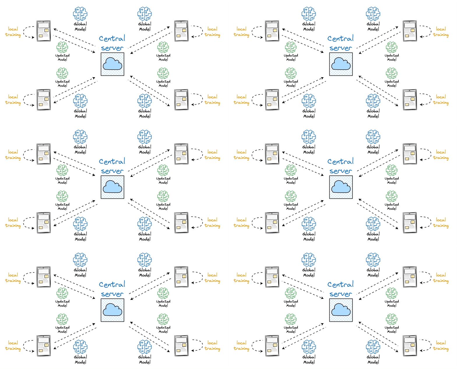
    <link href="https://www.dilawar.ai/2021/08/04/Federated%20Learning/"/>
    <id>https://www.dilawar.ai/2021/08/04/Federated%20Learning/</id>
    <published>2021-08-04T12:09:17.000Z</published>
    <updated>2026-10-28T18:47:53.825Z</updated>
    
    <content type="html"><![CDATA[<div style="display: flex; justify-content: space-between;"><p><img alt="Federated learning: devices train locally and exchange model updates with a central server." src="/images/federated.gif"/></p></div><p>Federated learning was a large part of my bachelor thesis. I wasinterested in training a shared model when the data stays with thepeople or devices that collected it. Building <ahref="https://github.com/dilawarm/federated">an implementation</a> for<a href="https://ntnuopen.ntnu.no/ntnu-xmlui/handle/11250/2778055">thethesis</a> also led me to study unreliable clients, malicious updates,and privacy.</p><h2 id="what-federated-learning-is">What federated learning is</h2><p>A centralized training setup brings the training data together. Infederated learning, clients train locally and send model updates to aserver, which combines them into a shared model. The raw data stays onthe clients, although the updates can still reveal information aboutit.</p><p>For a dataset of <span class="math inline">\(N\)</span> examples, acentralized training objective can be written as:</p><p><span class="math display">\[\min_{w \in \mathbb{R}^d} F(w) =\frac{1}{N} \sum_{i=1}^N \ell(x_{i}, y_{i}; w)\]</span></p><p>When the data is divided among clients, we can express that objectiveas a weighted sum of local losses:</p><p><span class="math display">\[F(w) = \sum_{k=1}^K\frac{n_{k}}{n_{\text{total}}} F_{k}(w)\]</span></p><p>where each client <span class="math inline">\(k\)</span> holds itsown local loss <span class="math inline">\(F_k\)</span> over <spanclass="math inline">\(n_k\)</span> data points.</p><p>A training round follows these steps:</p><ol type="1"><li>The server sends the current model to all clients.</li><li>Each client trains locally on its own data for a bit.</li><li>Clients send their updates back, never their data.</li><li>The server aggregates the updates into a new global model.</li></ol><p>Repeating these rounds lets the model learn from several clientswithout collecting their raw training examples on the server.</p><h2 id="aggregation-methods">Aggregation methods</h2><h3 id="fedsgd">FedSGD</h3><p>In FedSGD, clients compute gradients at the current global weightsand send them to the server. The server combines the gradients and takesan update step:</p><p><span class="math display">\[w^{t+1} = w^t - \eta \sum_{k=1}^K\frac{n_{k}}{n_{\text{total}}} \nabla F_{k}(w^t)\]</span></p><p>This requires communication for every global update, which can beexpensive when clients have slow or unreliable connections.</p><h3 id="fedavg">FedAvg</h3><p>FedAvg allows each client to take several local training steps beforesending its model back. The server then averages the resultingweights:</p><p><span class="math display">\[w^{t+1} = \sum_{k=1}^K\frac{n_{k}}{n_{\text{total}}} w_{k}^t\]</span></p><p>Taking more steps locally reduces communication, but clients may movein different directions if their data distributions differ. The numberof local steps becomes an important part of tuning the trainingprocess.</p><h2 id="robust-aggregation">Robust aggregation</h2><p>A client may send an incorrect update because of a software bug or anattempt to damage the model. A few extreme updates can pull anarithmetic mean far from the other clients’ results.</p><h3 id="geometric-median">Geometric median</h3><p>The geometric median is less sensitive to extreme updates. It finds apoint that minimizes the weighted sum of distances to the clientupdates:</p><p><span class="math display">\[\min_{z} \sum_{k=1}^m \alpha_{k} \|w_{k}- z\|\]</span></p><p>A smoothed form of the Weiszfeld algorithm approximates ititeratively:</p><p><span class="math display">\[z^{(i+1)} = \frac{\sum_{k=1}^m\beta_{k}^{(i)} w_{k}}{\sum_{k=1}^m \beta_{k}^{(i)}}, \quad\beta_{k}^{(i)} = \frac{\alpha_{k}}{\max\{\nu, \|w_{k} -z^{(i)}\|\}}\]</span></p><p>Updates farther from the current estimate receive less weight in thenext iteration. This reduces their influence, although it doesn’t makeevery kind of malicious update harmless.</p><h2 id="differential-privacy">Differential privacy</h2><p>Keeping raw data on a device doesn’t by itself guarantee privacy. Aserver may be able to infer information about training examples from theupdates it receives. Differential privacy gives us a way to bound howmuch the output can reveal.</p><h3 id="the-definition">The definition</h3><p>A mechanism <span class="math inline">\(\mathcal{M}\)</span> is <spanclass="math inline">\((\epsilon, \delta)\)</span>-differentially privateif, for any two datasets <span class="math inline">\(D\)</span> and<span class="math inline">\(D&#39;\)</span> that differ by onerecord:</p><p><span class="math display">\[\Pr(\mathcal{M}(D) \in S) \leqe^\epsilon \Pr(\mathcal{M}(D&#39;) \in S) + \delta\]</span></p><p>For the definition above, changing one record has a bounded effect onthe distribution of outputs. Smaller <spanclass="math inline">\(\epsilon\)</span> means a stronger bound when theother conditions are held fixed. The noise level, sampling procedure,and number of training rounds all affect the overall guarantee.</p><h3 id="adding-dp-to-fedavg">Adding DP to FedAvg</h3><p>The example here applies clipping and noise to each client’s modelupdate. These are the two operations, written for an update vector <spanclass="math inline">\(g_k\)</span>:</p><ol type="1"><li><p>Clip the update to a maximum norm: <spanclass="math display">\[\tilde{g}_{k} = \frac{g_{k}}{\max(1,\|g_{k}\|_{2} / C)}\]</span></p></li><li><p>Add Gaussian noise: <span class="math display">\[\hat{g}_k =\tilde{g}_k + \mathcal{N}(0, \sigma^2 C^2 \mathbf{I})\]</span></p></li></ol><p>The clipping and noise operations can be written in NumPy:</p><figure tabindex="0" role="region" aria-label="Code example 1" data-scroll-region class="highlight python"><table role="presentation"><tr><td class="gutter" aria-hidden="true"><pre><span class="line">1</span><br><span class="line">2</span><br><span class="line">3</span><br><span class="line">4</span><br><span class="line">5</span><br><span class="line">6</span><br><span class="line">7</span><br><span class="line">8</span><br><span class="line">9</span><br></pre></td><td class="code"><pre><span class="line"><span class="keyword">import</span> numpy <span class="keyword">as</span> np</span><br><span class="line"></span><br><span class="line"><span class="keyword">def</span> <span class="title function_">dp_clip_and_noise</span>(<span class="params">grad: np.ndarray, clip_norm: <span class="built_in">float</span> = <span class="number">1.0</span>, noise_multiplier: <span class="built_in">float</span> = <span class="number">1.0</span></span>) -&gt; np.ndarray:</span><br><span class="line">    norm = np.linalg.norm(grad)</span><br><span class="line">    <span class="keyword">if</span> norm &gt; clip_norm:</span><br><span class="line">        grad = (grad / norm) * clip_norm</span><br><span class="line">    noise_std = noise_multiplier * clip_norm</span><br><span class="line">    noise = np.random.normal(loc=<span class="number">0.0</span>, scale=noise_std, size=grad.shape)</span><br><span class="line">    <span class="keyword">return</span> grad + noise</span><br></pre></td></tr></table></figure><p>This function illustrates the mechanism, but it doesn’t calculate aprivacy guarantee. That requires choosing what is protected, calibratingthe noise, and accounting for repeated rounds. The <ahref="https://www.tensorflow.org/federated/tutorials/federated_learning_with_differential_privacy">TensorFlowFederated tutorial</a> works through training with user-leveldifferential privacy and privacy accounting.</p><h2 id="homomorphic-encryption">Homomorphic encryption</h2><p>Homomorphic encryption addresses a different question: can the servercombine updates without reading each one? Clients encrypt their updates,and the server performs the aggregation on ciphertexts.</p><h3 id="how-it-works">How it works</h3><p>For an additive homomorphic scheme, an operation on ciphertextscorresponds to addition of the underlying values. We can write thatrelationship schematically as:</p><p><span class="math display">\[\text{Enc}(a) \oplus \text{Enc}(b) =\text{Enc}(a + b)\]</span></p><p>For federated learning the workflow becomes:</p><ol type="1"><li>Each client encrypts its update: <span class="math inline">\(c_k =\text{Enc}(w_k)\)</span>.</li><li>The server sums the ciphertexts: <spanclass="math inline">\(c_{\text{sum}} = \sum_{k=1}^K c_k\)</span>.</li><li>Whoever holds the decryption key recovers <spanclass="math inline">\(\sum_k w_k\)</span>.</li></ol><p>With an abstract encryption backend, summing encrypted updates mightlook like this:</p><figure tabindex="0" role="region" aria-label="Code example 2" data-scroll-region class="highlight python"><table role="presentation"><tr><td class="gutter" aria-hidden="true"><pre><span class="line">1</span><br><span class="line">2</span><br><span class="line">3</span><br><span class="line">4</span><br><span class="line">5</span><br><span class="line">6</span><br><span class="line">7</span><br><span class="line">8</span><br><span class="line">9</span><br><span class="line">10</span><br><span class="line">11</span><br><span class="line">12</span><br><span class="line">13</span><br><span class="line">14</span><br><span class="line">15</span><br></pre></td><td class="code"><pre><span class="line"><span class="keyword">from</span> typing <span class="keyword">import</span> <span class="type">Any</span>, Protocol</span><br><span class="line"></span><br><span class="line"><span class="keyword">class</span> <span class="title class_">HEContext</span>(<span class="title class_ inherited__">Protocol</span>):</span><br><span class="line">    <span class="keyword">def</span> <span class="title function_">encrypt_zeros</span>(<span class="params">self</span>) -&gt; <span class="type">Any</span>: ...</span><br><span class="line">    <span class="keyword">def</span> <span class="title function_">homomorphic_add</span>(<span class="params">self, a: <span class="type">Any</span>, b: <span class="type">Any</span></span>) -&gt; <span class="type">Any</span>: ...</span><br><span class="line">    <span class="keyword">def</span> <span class="title function_">decrypt</span>(<span class="params">self, ciphertext: <span class="type">Any</span></span>) -&gt; <span class="type">Any</span>: ...</span><br><span class="line"></span><br><span class="line"><span class="keyword">def</span> <span class="title function_">homomorphic_aggregate</span>(<span class="params">encrypted_updates: <span class="built_in">list</span>[<span class="type">Any</span>], he_context: HEContext</span>) -&gt; <span class="type">Any</span>:</span><br><span class="line">    c_sum = he_context.encrypt_zeros()</span><br><span class="line">    <span class="keyword">for</span> c_u <span class="keyword">in</span> encrypted_updates:</span><br><span class="line">        c_sum = he_context.homomorphic_add(c_sum, c_u)</span><br><span class="line">    <span class="keyword">return</span> c_sum</span><br><span class="line"></span><br><span class="line"><span class="keyword">def</span> <span class="title function_">decrypt_sum</span>(<span class="params">c_sum: <span class="type">Any</span>, he_context: HEContext</span>) -&gt; <span class="type">Any</span>:</span><br><span class="line">    <span class="keyword">return</span> he_context.decrypt(c_sum)</span><br></pre></td></tr></table></figure><h2 id="putting-it-all-together">Putting it all together</h2><p>The following example combines local training, clipping, noise, andaveraging. It is a small demonstration of those operations, without theprivacy accounting needed for a complete private training system:</p><figure tabindex="0" role="region" aria-label="Code example 3" data-scroll-region class="highlight python"><table role="presentation"><tr><td class="gutter" aria-hidden="true"><pre><span class="line">1</span><br><span class="line">2</span><br><span class="line">3</span><br><span class="line">4</span><br><span class="line">5</span><br><span class="line">6</span><br><span class="line">7</span><br><span class="line">8</span><br><span class="line">9</span><br><span class="line">10</span><br><span class="line">11</span><br><span class="line">12</span><br><span class="line">13</span><br><span class="line">14</span><br><span class="line">15</span><br><span class="line">16</span><br><span class="line">17</span><br><span class="line">18</span><br><span class="line">19</span><br><span class="line">20</span><br><span class="line">21</span><br><span class="line">22</span><br><span class="line">23</span><br><span class="line">24</span><br><span class="line">25</span><br><span class="line">26</span><br><span class="line">27</span><br><span class="line">28</span><br><span class="line">29</span><br><span class="line">30</span><br><span class="line">31</span><br><span class="line">32</span><br><span class="line">33</span><br><span class="line">34</span><br><span class="line">35</span><br><span class="line">36</span><br></pre></td><td class="code"><pre><span class="line"><span class="keyword">import</span> numpy <span class="keyword">as</span> np</span><br><span class="line"></span><br><span class="line"><span class="keyword">def</span> <span class="title function_">local_train</span>(<span class="params">model_params, local_data, epochs: <span class="built_in">int</span> = <span class="number">1</span>, lr: <span class="built_in">float</span> = <span class="number">0.01</span></span>):</span><br><span class="line">    w = np.copy(model_params)</span><br><span class="line">    <span class="keyword">for</span> _ <span class="keyword">in</span> <span class="built_in">range</span>(epochs):</span><br><span class="line">        grad = compute_gradient(w, local_data)</span><br><span class="line">        w = w - lr * grad</span><br><span class="line">    <span class="keyword">return</span> w</span><br><span class="line"></span><br><span class="line"><span class="keyword">def</span> <span class="title function_">compute_gradient</span>(<span class="params">w, data</span>):</span><br><span class="line">    X, y = data</span><br><span class="line">    preds = X @ w</span><br><span class="line">    errs = preds - y</span><br><span class="line">    <span class="keyword">return</span> (X.T @ errs) / <span class="built_in">len</span>(X)</span><br><span class="line"></span><br><span class="line"><span class="keyword">def</span> <span class="title function_">federated_round</span>(<span class="params">global_params, clients_data, clip_norm: <span class="built_in">float</span>, noise_multiplier: <span class="built_in">float</span></span>):</span><br><span class="line">    updated_params = []</span><br><span class="line">    <span class="keyword">for</span> local_data <span class="keyword">in</span> clients_data:</span><br><span class="line">        w_k = local_train(global_params, local_data)</span><br><span class="line">        grad_k = w_k - global_params</span><br><span class="line">        grad_k_dp = dp_clip_and_noise(grad_k, clip_norm, noise_multiplier)</span><br><span class="line">        updated_params.append(global_params + grad_k_dp)</span><br><span class="line">    <span class="keyword">return</span> np.mean(updated_params, axis=<span class="number">0</span>)</span><br><span class="line"></span><br><span class="line"><span class="keyword">if</span> __name__ == <span class="string">&quot;__main__&quot;</span>:</span><br><span class="line">    w_global = np.zeros(<span class="number">2</span>)</span><br><span class="line">    </span><br><span class="line">    clients_data = [</span><br><span class="line">        (np.array([[<span class="number">1</span>, <span class="number">2</span>], [<span class="number">0</span>, <span class="number">1</span>]]), np.array([<span class="number">1.0</span>, <span class="number">0.0</span>])),</span><br><span class="line">        (np.array([[<span class="number">3</span>, <span class="number">2</span>], [<span class="number">4</span>, <span class="number">1</span>]]), np.array([<span class="number">2.0</span>, <span class="number">3.0</span>])),</span><br><span class="line">        (np.array([[<span class="number">10</span>, <span class="number">2</span>], [<span class="number">8</span>, <span class="number">2</span>]]), np.array([<span class="number">4.0</span>, <span class="number">5.0</span>])),</span><br><span class="line">    ]</span><br><span class="line">    </span><br><span class="line">    <span class="keyword">for</span> t <span class="keyword">in</span> <span class="built_in">range</span>(<span class="number">5</span>):</span><br><span class="line">        w_global = federated_round(w_global, clients_data, clip_norm=<span class="number">2.0</span>, noise_multiplier=<span class="number">0.5</span>)</span><br><span class="line">        <span class="built_in">print</span>(<span class="string">f&quot;Round <span class="subst">&#123;t&#125;</span>, global params = <span class="subst">&#123;w_global&#125;</span>&quot;</span>)</span><br></pre></td></tr></table></figure><p>Robust aggregation, differential privacy, and homomorphic encryptionaddress different threats. Combining them takes care: an aggregationmethod that needs to inspect individual updates may be difficult toapply when those updates are encrypted.</p><h2 id="what-broke-when-i-built-this">What broke when I built this</h2><p>The implementation brought up several issues that were easy tooverlook in the equations.</p><p><strong>Non-IID data</strong> was the biggest difficulty. Clientsdon’t all collect examples from the same distribution, so training onone client’s data can move the model in a different direction fromtraining on another’s.</p><p><strong>Client dropout</strong> meant the server couldn’t assumeeveryone would finish a round. Phones go offline and apps close, so theaggregation process needed a policy for incomplete participation.</p><p><strong>Privacy and accuracy</strong> needed to be consideredtogether. Noise changes the updates used for training, while encryptionadds computation and communication costs. Choosing those settingsaffected both the protection and the usefulness of the model.</p><h2 id="what-stuck-with-me">What stuck with me</h2><p>Federated learning gave me a useful example of how an optimizationmethod changes when it has to run across separate devices. The averagingstep is small, but the system also needs to account for different datadistributions, missing clients, and information that can leak throughupdates.</p><p>I found the interaction between privacy and robustness especiallyinteresting. Preventing a server from seeing an update and helping itidentify a bad update can pull the design in different directions. Theright combination depends on which parties the system trusts and whatattacks it is meant to resist.</p><p><a href="https://ntnuopen.ntnu.no/ntnu-xmlui/handle/11250/2778055">Mythesis</a> has the fuller discussion, and <ahref="https://github.com/dilawarm/federated">the repository</a> containsthe implementation.</p>]]></content>


    <summary type="html">&lt;div style=&quot;display: flex; justify-content: space-between;&quot;&gt;
&lt;p&gt;&lt;img alt=&quot;Federated learning: devices train locally and exchange model</summary>


    <category term="Cryptography" scheme="https://www.dilawar.ai/tags/Cryptography/"/>
    
    <category term="Machine Learning" scheme="https://www.dilawar.ai/tags/Machine-Learning/"/>
    
    <category term="Distributed Systems" scheme="https://www.dilawar.ai/tags/Distributed-Systems/"/>
    
  </entry>
  
  <entry>
    <title>Statistical Learning: Essential Mathematics</title>
    <link href="https://www.dilawar.ai/2021/07/21/Statistical%20Learning:%20Essential%20Mathematics/"/>
    <id>https://www.dilawar.ai/2021/07/21/Statistical%20Learning:%20Essential%20Mathematics/</id>
    <published>2021-07-21T10:11:21.000Z</published>
    <updated>2026-10-28T18:47:53.825Z</updated>
    
    <content type="html"><![CDATA[<div style="display: flex; justify-content: space-between;"><p><img alt="Kermit celebrating with the caption “Yay statistics”." src="/images/stats.gif"/></p></div><p>Taking <ahref="https://www.ntnu.edu/studies/courses/TMA4268#tab=omEmnet">TMA4268at NTNU</a> helped me understand several choices I’d been making byhabit when training models. I had been more interested in trying neuralnetworks than in studying statistics, but the course gave me better waysto think about model error and uncertainty.</p><h2 id="the-math-underneath-the-methods">The math underneath themethods</h2><p>Statistical learning studies how we learn from samples and how wellthe resulting models might perform on new data. Ideas such as maximumlikelihood, hypothesis testing, and the bias-variance decomposition helpmake the assumptions behind a method explicit.</p><p>One way to describe a supervised learning problem is with an inputspace <span class="math inline">\(X\)</span>, an output space <spanclass="math inline">\(Y\)</span>, and a distribution <spanclass="math inline">\(P\)</span> over pairs of inputs and outputs. Wewant a function <span class="math inline">\(f: X \to Y\)</span> thatminimizes the expected risk:</p><p><span class="math display">\[R(f) = \int_{X \times Y} L(f(x), y) \,dP(x, y)\]</span></p><p>Here <span class="math inline">\(L\)</span> measures the cost of aprediction. Linear regression, logistic regression, and neural networkscan all be studied within this framework, even though they use differentfunctions and losses.</p><h2 id="why-bother-with-statistics">Why bother with statistics</h2><p>Fitting a model leaves several questions unanswered. We may want toknow how uncertain a coefficient is, whether a feature adds usefulinformation, or how much a result changes across samples. Statisticalmethods give us ways to investigate these questions, provided we checktheir assumptions.</p><p>This linear regression example calculates coefficient estimates,standard errors, and p-values:</p><figure tabindex="0" role="region" aria-label="Code example 1" data-scroll-region class="highlight python"><table role="presentation"><tr><td class="gutter" aria-hidden="true"><pre><span class="line">1</span><br><span class="line">2</span><br><span class="line">3</span><br><span class="line">4</span><br><span class="line">5</span><br><span class="line">6</span><br><span class="line">7</span><br><span class="line">8</span><br><span class="line">9</span><br><span class="line">10</span><br><span class="line">11</span><br><span class="line">12</span><br><span class="line">13</span><br><span class="line">14</span><br><span class="line">15</span><br><span class="line">16</span><br><span class="line">17</span><br><span class="line">18</span><br><span class="line">19</span><br><span class="line">20</span><br><span class="line">21</span><br><span class="line">22</span><br><span class="line">23</span><br></pre></td><td class="code"><pre><span class="line"><span class="keyword">import</span> numpy <span class="keyword">as</span> np</span><br><span class="line"><span class="keyword">from</span> scipy <span class="keyword">import</span> stats</span><br><span class="line"></span><br><span class="line"><span class="keyword">def</span> <span class="title function_">fit_linear_model</span>(<span class="params">X: np.ndarray, y: np.ndarray</span>) -&gt; <span class="built_in">dict</span>:</span><br><span class="line">    X = np.column_stack([np.ones(X.shape[<span class="number">0</span>]), X])</span><br><span class="line">    </span><br><span class="line">    beta = np.linalg.inv(X.T @ X) @ X.T @ y</span><br><span class="line">    </span><br><span class="line">    n = X.shape[<span class="number">0</span>]</span><br><span class="line">    y_pred = X @ beta</span><br><span class="line">    residuals = y - y_pred</span><br><span class="line">    mse = np.<span class="built_in">sum</span>(residuals**<span class="number">2</span>) / (n - X.shape[<span class="number">1</span>])</span><br><span class="line">    var_beta = mse * np.linalg.inv(X.T @ X)</span><br><span class="line">    se = np.sqrt(np.diag(var_beta))</span><br><span class="line">    </span><br><span class="line">    t_stats = beta / se</span><br><span class="line">    p_values = <span class="number">2</span> * (<span class="number">1</span> - stats.t.cdf(np.<span class="built_in">abs</span>(t_stats), n - X.shape[<span class="number">1</span>]))</span><br><span class="line">    </span><br><span class="line">    <span class="keyword">return</span> &#123;</span><br><span class="line">        <span class="string">&#x27;coefficients&#x27;</span>: beta,</span><br><span class="line">        <span class="string">&#x27;std_errors&#x27;</span>: se,</span><br><span class="line">        <span class="string">&#x27;p_values&#x27;</span>: p_values,</span><br><span class="line">    &#125;</span><br></pre></td></tr></table></figure><p>The standard errors describe uncertainty in the coefficient estimatesunder the regression model’s assumptions. The p-values test whether acoefficient differs from zero within that model; they don’t establishthat a feature causes the outcome.</p><h2 id="the-bias-variance-decomposition">The bias-variancedecomposition</h2><p>The bias-variance decomposition was especially useful forunderstanding squared prediction error:</p><p><span class="math display">\[E[(Y - \hat{f}(X))^2] =\text{Var}(\hat{f}(X)) + [\text{Bias}(\hat{f}(X))]^2 +\sigma^2\]</span></p><p>The three terms describe variation across training samples,systematic error in the average prediction, and noise in the outcome. Amore flexible model can reduce bias while becoming more sensitive to theparticular sample used to train it. This helps explain why reducingtraining error doesn’t always improve predictions on new data.</p><h2 id="combining-ml-with-statistical-rigor">Combining ML withstatistical rigor</h2><p>Cross-validation gives several scores, and looking at their spreadtells us more than reporting the mean alone. The example below alsocalculates a simple t-based interval, whose assumptions need care:</p><figure tabindex="0" role="region" aria-label="Code example 2" data-scroll-region class="highlight python"><table role="presentation"><tr><td class="gutter" aria-hidden="true"><pre><span class="line">1</span><br><span class="line">2</span><br><span class="line">3</span><br><span class="line">4</span><br><span class="line">5</span><br><span class="line">6</span><br><span class="line">7</span><br><span class="line">8</span><br><span class="line">9</span><br><span class="line">10</span><br><span class="line">11</span><br><span class="line">12</span><br><span class="line">13</span><br><span class="line">14</span><br><span class="line">15</span><br><span class="line">16</span><br><span class="line">17</span><br><span class="line">18</span><br><span class="line">19</span><br><span class="line">20</span><br><span class="line">21</span><br><span class="line">22</span><br><span class="line">23</span><br><span class="line">24</span><br><span class="line">25</span><br></pre></td><td class="code"><pre><span class="line"><span class="keyword">from</span> sklearn.model_selection <span class="keyword">import</span> KFold</span><br><span class="line"><span class="keyword">import</span> numpy <span class="keyword">as</span> np</span><br><span class="line"><span class="keyword">from</span> scipy <span class="keyword">import</span> stats</span><br><span class="line"></span><br><span class="line"><span class="keyword">def</span> <span class="title function_">statistical_cross_validate</span>(<span class="params">model, X, y, n_splits: <span class="built_in">int</span> = <span class="number">5</span></span>):</span><br><span class="line">    kf = KFold(n_splits=n_splits, shuffle=<span class="literal">True</span>)</span><br><span class="line">    scores = []</span><br><span class="line">    </span><br><span class="line">    <span class="keyword">for</span> train_idx, test_idx <span class="keyword">in</span> kf.split(X):</span><br><span class="line">        X_train, X_test = X[train_idx], X[test_idx]</span><br><span class="line">        y_train, y_test = y[train_idx], y[test_idx]</span><br><span class="line">        </span><br><span class="line">        model.fit(X_train, y_train)</span><br><span class="line">        scores.append(model.score(X_test, y_test))</span><br><span class="line">    </span><br><span class="line">    mean_score = np.mean(scores)</span><br><span class="line">    ci = stats.t.interval(</span><br><span class="line">        <span class="number">0.95</span>, <span class="built_in">len</span>(scores) - <span class="number">1</span>, loc=mean_score, scale=stats.sem(scores)</span><br><span class="line">    )</span><br><span class="line">    </span><br><span class="line">    <span class="keyword">return</span> &#123;</span><br><span class="line">        <span class="string">&#x27;mean_score&#x27;</span>: mean_score,</span><br><span class="line">        <span class="string">&#x27;confidence_interval&#x27;</span>: ci,</span><br><span class="line">        <span class="string">&#x27;std_score&#x27;</span>: np.std(scores),</span><br><span class="line">    &#125;</span><br></pre></td></tr></table></figure><p>The calculation treats the fold scores as independent, even thoughtheir training sets overlap. That can make the interval too narrow, so Iwouldn’t use it as a reliable 95% confidence interval or as proof thatone model is better. Scikit-learn’s <ahref="https://scikit-learn.org/stable/auto_examples/model_selection/plot_grid_search_stats.html">exampleon statistical model comparison</a> explains the dependence and shows acorrected comparison.</p><h2 id="what-i-took-from-the-course">Choosing a baseline</h2><p>The course made me more willing to start with a linear or generalizedlinear model and examine its errors before adding complexity. That givesme a baseline I can understand. If a neural network improves on it, Istill want to know how stable the improvement is and where the modelfails.</p><p>I now pay more attention to how a result was measured and whatassumptions support it. A good score is useful, but I also want tounderstand how much confidence I can place in it.</p>]]></content>


    <summary type="html">&lt;div style=&quot;display: flex; justify-content: space-between;&quot;&gt;
&lt;p&gt;&lt;img alt=&quot;Kermit celebrating with the caption “Yay statistics”.&quot;</summary>


    <category term="Mathematics" scheme="https://www.dilawar.ai/tags/Mathematics/"/>
    
    <category term="Machine Learning" scheme="https://www.dilawar.ai/tags/Machine-Learning/"/>
    
    <category term="Statistical Learning" scheme="https://www.dilawar.ai/tags/Statistical-Learning/"/>
    
  </entry>
  
  <entry>
    <title>Abstract Algebra in Modern Cryptography</title>
    <link href="https://www.dilawar.ai/2021/05/05/Abstract%20Algebra%20in%20Modern%20Cryptography/"/>
    <id>https://www.dilawar.ai/2021/05/05/Abstract%20Algebra%20in%20Modern%20Cryptography/</id>
    <published>2021-05-05T10:11:21.000Z</published>
    <updated>2026-10-28T18:47:53.825Z</updated>
    
    <content type="html"><![CDATA[<div style="display: flex; justify-content: space-between;"><p><img alt="Animation illustrating transformations in group theory." src="/images/algebra.gif"/></p></div><p>Groups, rings, and fields made more sense to me once I startedreading about cryptography. During <ahref="https://www.ntnu.edu/studies/courses/TMA4150#tab=omEmnet">Algebraat NTNU</a>, I’d often wondered what I would use them for. Cryptographygave me concrete examples of why those definitions mattered.</p><h2 id="the-basics">The basics</h2><p>A group <span class="math inline">\((G, \cdot)\)</span> is a set withan operation that satisfies four conditions. Combining two elementsgives another element in the set, and changing the grouping of anexpression doesn’t change its result. There is also an identity element,which leaves other elements unchanged, and every element has an inverse.These conditions give us a common way to study operations that mightotherwise look unrelated.</p><p>A homomorphism maps one group to another while preserving theoperation. Applying the map after combining two elements gives the sameresult as mapping them first and then combining them:</p><p><span class="math display">\[\phi : G \rightarrow H \text{ such that} \phi(a \cdot b) = \phi(a) \star \phi(b)\]</span></p><p>This idea is useful in cryptography because it gives us a way torelate operations on messages to operations on ciphertexts. A Pythonwrapper for such a map might look like this, although the wrapper itselfdoesn’t check that the map preserves the operation:</p><figure tabindex="0" role="region" aria-label="Code example 1" data-scroll-region class="highlight python"><table role="presentation"><tr><td class="gutter" aria-hidden="true"><pre><span class="line">1</span><br><span class="line">2</span><br><span class="line">3</span><br><span class="line">4</span><br><span class="line">5</span><br><span class="line">6</span><br><span class="line">7</span><br><span class="line">8</span><br><span class="line">9</span><br><span class="line">10</span><br><span class="line">11</span><br></pre></td><td class="code"><pre><span class="line"><span class="keyword">from</span> typing <span class="keyword">import</span> TypeVar, <span class="type">Generic</span>, <span class="type">Callable</span></span><br><span class="line"></span><br><span class="line">T = TypeVar(<span class="string">&#x27;T&#x27;</span>)</span><br><span class="line">S = TypeVar(<span class="string">&#x27;S&#x27;</span>)</span><br><span class="line"></span><br><span class="line"><span class="keyword">class</span> <span class="title class_">Homomorphism</span>(<span class="type">Generic</span>[T, S]):</span><br><span class="line">    <span class="keyword">def</span> <span class="title function_">__init__</span>(<span class="params">self, mapping_func: <span class="type">Callable</span>[[T], S]</span>):</span><br><span class="line">        <span class="variable language_">self</span>.mapping_func = mapping_func</span><br><span class="line">        </span><br><span class="line">    <span class="keyword">def</span> <span class="title function_">map</span>(<span class="params">self, element: T</span>) -&gt; S:</span><br><span class="line">        <span class="keyword">return</span> <span class="variable language_">self</span>.mapping_func(element)</span><br></pre></td></tr></table></figure><h2 id="computing-on-encrypted-data">Computing on encrypted data</h2><p>Homomorphic encryption allows certain calculations on encryptedvalues. For a scheme that supports both addition and multiplication, therelationship can be written schematically as:</p><p><span class="math display">\[E(x + y) = E(x) \oplus E(y) \quad\text{and} \quad E(x \cdot y) = E(x) \otimes E(y)\]</span></p><p>The operations on the right happen on ciphertexts, and decrypting theresult should recover the corresponding calculation on the originalvalues. This small example illustrates the additive relationship, but itis not secure encryption:</p><figure tabindex="0" role="region" aria-label="Code example 2" data-scroll-region class="highlight python"><table role="presentation"><tr><td class="gutter" aria-hidden="true"><pre><span class="line">1</span><br><span class="line">2</span><br><span class="line">3</span><br><span class="line">4</span><br><span class="line">5</span><br><span class="line">6</span><br><span class="line">7</span><br><span class="line">8</span><br><span class="line">9</span><br><span class="line">10</span><br><span class="line">11</span><br><span class="line">12</span><br></pre></td><td class="code"><pre><span class="line"><span class="keyword">from</span> dataclasses <span class="keyword">import</span> dataclass</span><br><span class="line"></span><br><span class="line"><span class="meta">@dataclass</span></span><br><span class="line"><span class="keyword">class</span> <span class="title class_">HomomorphicCipher</span>:</span><br><span class="line">    modulus: <span class="built_in">int</span></span><br><span class="line">    key: <span class="built_in">int</span></span><br><span class="line">    </span><br><span class="line">    <span class="keyword">def</span> <span class="title function_">encrypt</span>(<span class="params">self, message: <span class="built_in">int</span></span>) -&gt; <span class="built_in">int</span>:</span><br><span class="line">        <span class="keyword">return</span> (message * <span class="variable language_">self</span>.key) % <span class="variable language_">self</span>.modulus</span><br><span class="line">    </span><br><span class="line">    <span class="keyword">def</span> <span class="title function_">bulk_add</span>(<span class="params">self, ciphertexts: <span class="built_in">list</span>[<span class="built_in">int</span>]</span>) -&gt; <span class="built_in">int</span>:</span><br><span class="line">        <span class="keyword">return</span> <span class="built_in">sum</span>(ciphertexts) % <span class="variable language_">self</span>.modulus</span><br></pre></td></tr></table></figure><p>Schemes such as BFV, BGV, and CKKS need much more machinery to makethis useful and secure. The toy example only illustrates the property wewant to preserve.</p><h2 id="why-public-key-crypto-works-at-all">Why public-key crypto worksat all</h2><p>Public-key cryptography often relies on problems that are easy tocompute in one direction and difficult to reverse without extrainformation. One example is the discrete logarithm problem:</p><p><span class="math display">\[\text{Given } g^x \equiv h \pmod{p},\text{ find } x\]</span></p><p>Computing <span class="math inline">\(g^x \bmod p\)</span> isefficient, while recovering <span class="math inline">\(x\)</span> canbe difficult when the group and its parameters are chosen appropriately.Cryptographic protocols use that difference to let people exchangeinformation without also revealing their private keys.</p><p>RSA is related to the difficulty of factoring large semiprimes, whileelliptic curve cryptography uses the discrete logarithm problem inelliptic curve groups. The algebra helps us describe these constructionsand reason about their properties.</p><h2 id="looking-back">Reading cryptography papers</h2><p>When I went back to quotient groups and the other material from thecourse, I had a better reason to care about the details. The definitionswere giving me a way to follow cryptography papers that I couldn’t haveread before.</p>]]></content>


    <summary type="html">&lt;div style=&quot;display: flex; justify-content: space-between;&quot;&gt;
&lt;p&gt;&lt;img alt=&quot;Animation illustrating transformations in group theory.&quot;</summary>


    <category term="Mathematics" scheme="https://www.dilawar.ai/tags/Mathematics/"/>
    
    <category term="Cryptography" scheme="https://www.dilawar.ai/tags/Cryptography/"/>
    
    <category term="Algebra" scheme="https://www.dilawar.ai/tags/Algebra/"/>
    
  </entry>
  
  <entry>
    <title>Video Style Transfer: Coherence vs Quality</title>
    <link href="https://www.dilawar.ai/2020/12/14/Video%20Style%20Transfer:%20Coherence%20vs%20Quality/"/>
    <id>https://www.dilawar.ai/2020/12/14/Video%20Style%20Transfer:%20Coherence%20vs%20Quality/</id>
    <published>2020-12-14T19:47:24.000Z</published>
    <updated>2026-10-28T18:47:53.825Z</updated>
    
    <content type="html"><![CDATA[<div style="display: flex; justify-content: space-between;"><p><img src="/images/shrek_la_muse.gif" alt="Shrek styled with La Muse" /></p></div><p>The video style transfer project we built at NTNU began with aproblem I hadn’t appreciated from looking at still images. A frame couldlook good on its own and still look wrong when played beside the nextone. Getting the painted texture to follow the motion became a largepart of the work.</p><h2 id="why-its-harder-than-it-looks">Why it’s harder than it looks</h2><p>When style transfer processes each frame independently, it can placedifferent textures on the same part of a scene from one frame to thenext. Those changes appear as flicker during playback. We needed to keepthe frames consistent while preserving both the motion and the chosenstyle.</p><h3 id="the-math">The math</h3><p>A convolutional network provides features for comparing content andstyle. For a frame <span class="math inline">\(I_t\)</span>, we can usecontent features <span class="math inline">\(F_c\)</span> and stylefeatures <span class="math inline">\(F_s\)</span>, then add a temporalterm that measures changes between frames:</p><p><span class="math display">\[L_{total} = \alpha L_c + \beta L_s +\gamma L_{temporal}\]</span></p><p>Here <span class="math inline">\(L_c\)</span> measures contentdifferences, <span class="math inline">\(L_s\)</span> measures styledifferences, and <span class="math inline">\(L_{temporal}\)</span>measures inconsistency over time. The weights <spanclass="math inline">\(\alpha\)</span>, <spanclass="math inline">\(\beta\)</span>, and <spanclass="math inline">\(\gamma\)</span> control their relativeinfluence.</p><h2 id="making-it-smooth-over-time">Making it smooth over time</h2><p>A simple temporal loss penalizes differences between consecutivestylized frames <span class="math inline">\(S(I_{t-1})\)</span> and<span class="math inline">\(S(I_t)\)</span>:</p><p><span class="math display">\[L_{temporal} = \sum_{i,j} \| S(I_t) -S(I_{t-1}) \|\]</span></p><p>Comparing frames directly also penalizes real movement, so ourversion used optical flow to estimate where pixels had moved. We warpedthe previous stylized frame into the current frame’s coordinates beforecomparing them:</p><figure tabindex="0" role="region" aria-label="Code example 1" data-scroll-region class="highlight python"><table role="presentation"><tr><td class="gutter" aria-hidden="true"><pre><span class="line">1</span><br><span class="line">2</span><br><span class="line">3</span><br><span class="line">4</span><br><span class="line">5</span><br><span class="line">6</span><br><span class="line">7</span><br><span class="line">8</span><br><span class="line">9</span><br><span class="line">10</span><br><span class="line">11</span><br><span class="line">12</span><br><span class="line">13</span><br><span class="line">14</span><br><span class="line">15</span><br><span class="line">16</span><br><span class="line">17</span><br><span class="line">18</span><br><span class="line">19</span><br><span class="line">20</span><br><span class="line">21</span><br><span class="line">22</span><br><span class="line">23</span><br><span class="line">24</span><br><span class="line">25</span><br><span class="line">26</span><br><span class="line">27</span><br><span class="line">28</span><br><span class="line">29</span><br><span class="line">30</span><br><span class="line">31</span><br><span class="line">32</span><br><span class="line">33</span><br><span class="line">34</span><br><span class="line">35</span><br><span class="line">36</span><br><span class="line">37</span><br></pre></td><td class="code"><pre><span class="line"><span class="keyword">import</span> torch</span><br><span class="line"><span class="keyword">import</span> torch.nn <span class="keyword">as</span> nn</span><br><span class="line"><span class="keyword">import</span> torch.nn.functional <span class="keyword">as</span> F</span><br><span class="line"><span class="keyword">from</span> torch <span class="keyword">import</span> Tensor</span><br><span class="line"></span><br><span class="line"><span class="keyword">def</span> <span class="title function_">temporal_loss</span>(<span class="params">prev_frame: Tensor, curr_frame: Tensor, flow: Tensor, reduction: <span class="built_in">str</span> = <span class="string">&#x27;mean&#x27;</span></span>) -&gt; Tensor:</span><br><span class="line">    warped_prev = warp_frame(prev_frame, flow)</span><br><span class="line">    diff = torch.<span class="built_in">abs</span>(curr_frame - warped_prev)</span><br><span class="line">    </span><br><span class="line">    <span class="keyword">if</span> reduction == <span class="string">&#x27;mean&#x27;</span>:</span><br><span class="line">        <span class="keyword">return</span> torch.mean(diff)</span><br><span class="line">    <span class="keyword">elif</span> reduction == <span class="string">&#x27;sum&#x27;</span>:</span><br><span class="line">        <span class="keyword">return</span> torch.<span class="built_in">sum</span>(diff)</span><br><span class="line">    <span class="keyword">else</span>:</span><br><span class="line">        <span class="keyword">raise</span> ValueError(<span class="string">f&quot;Unsupported reduction method: <span class="subst">&#123;reduction&#125;</span>&quot;</span>)</span><br><span class="line"></span><br><span class="line"><span class="keyword">def</span> <span class="title function_">warp_frame</span>(<span class="params">frame: Tensor, flow: Tensor</span>) -&gt; Tensor:</span><br><span class="line">    B, C, H, W = frame.shape</span><br><span class="line">    </span><br><span class="line">    grid_y, grid_x = torch.meshgrid(</span><br><span class="line">        torch.arange(H, device=frame.device),</span><br><span class="line">        torch.arange(W, device=frame.device),</span><br><span class="line">        indexing=<span class="string">&#x27;ij&#x27;</span></span><br><span class="line">    )</span><br><span class="line">    </span><br><span class="line">    flow_grid = torch.stack([</span><br><span class="line">        <span class="number">2</span> * (grid_x + flow[:, <span class="number">0</span>]) / (W - <span class="number">1</span>) - <span class="number">1</span>,</span><br><span class="line">        <span class="number">2</span> * (grid_y + flow[:, <span class="number">1</span>]) / (H - <span class="number">1</span>) - <span class="number">1</span></span><br><span class="line">    ], dim=-<span class="number">1</span>)</span><br><span class="line">    </span><br><span class="line">    <span class="keyword">return</span> F.grid_sample(</span><br><span class="line">        frame,</span><br><span class="line">        flow_grid.permute(<span class="number">0</span>, <span class="number">2</span>, <span class="number">3</span>, <span class="number">1</span>),</span><br><span class="line">        mode=<span class="string">&#x27;bilinear&#x27;</span>,</span><br><span class="line">        padding_mode=<span class="string">&#x27;border&#x27;</span>,</span><br><span class="line">        align_corners=<span class="literal">True</span></span><br><span class="line">    )</span><br></pre></td></tr></table></figure><p>This encourages a point in the scene to keep a consistent appearanceas it moves, rather than encouraging every pixel to stay unchanged.</p><h2 id="approaches-we-tried">Approaches we tried</h2><h3 id="frame-by-frame-gatys">Frame-by-frame Gatys</h3><p>We first applied <ahref="https://arxiv.org/abs/1508.06576">Gatys-style</a> optimization toeach frame independently. The resulting flicker gave us a usefulbaseline for judging whether later changes improved consistency.</p><h3 id="optical-flow-constraints-ruder">Optical flow constraints(Ruder)</h3><p><a href="https://arxiv.org/abs/1604.08610">Ruder’s approach</a> usesoptical flow to constrain how the stylized image changes between frames.It improved consistency, but estimating the flow added computation andmade the implementation more involved.</p><h3 id="feedforward-networks-with-instance-normalization">Feedforwardnetworks with instance normalization</h3><p>Optimization-based methods repeatedly update an image to minimize theloss. <a href="https://arxiv.org/abs/1603.08155">Johnson et al.</a>instead train a feedforward network to produce the stylized image in onepass. We used instance normalization in our version:</p><figure tabindex="0" role="region" aria-label="Code example 2" data-scroll-region class="highlight python"><table role="presentation"><tr><td class="gutter" aria-hidden="true"><pre><span class="line">1</span><br><span class="line">2</span><br><span class="line">3</span><br><span class="line">4</span><br><span class="line">5</span><br><span class="line">6</span><br><span class="line">7</span><br><span class="line">8</span><br><span class="line">9</span><br><span class="line">10</span><br><span class="line">11</span><br></pre></td><td class="code"><pre><span class="line"><span class="keyword">class</span> <span class="title class_">InstanceNorm</span>(nn.Module):</span><br><span class="line">    <span class="keyword">def</span> <span class="title function_">__init__</span>(<span class="params">self, dim: <span class="built_in">int</span>, eps: <span class="built_in">float</span> = <span class="number">1e-8</span></span>) -&gt; <span class="literal">None</span>:</span><br><span class="line">        <span class="built_in">super</span>().__init__()</span><br><span class="line">        <span class="variable language_">self</span>.scale = nn.Parameter(torch.ones(dim))</span><br><span class="line">        <span class="variable language_">self</span>.shift = nn.Parameter(torch.zeros(dim))</span><br><span class="line">        <span class="variable language_">self</span>.eps = eps</span><br><span class="line">        </span><br><span class="line">    <span class="keyword">def</span> <span class="title function_">forward</span>(<span class="params">self, x: Tensor</span>) -&gt; Tensor:</span><br><span class="line">        mean = x.mean(dim=(<span class="number">2</span>, <span class="number">3</span>), keepdim=<span class="literal">True</span>)</span><br><span class="line">        std = x.std(dim=(<span class="number">2</span>, <span class="number">3</span>), keepdim=<span class="literal">True</span>) + <span class="variable language_">self</span>.eps</span><br><span class="line">        <span class="keyword">return</span> <span class="variable language_">self</span>.scale[<span class="literal">None</span>, :, <span class="literal">None</span>, <span class="literal">None</span>] * (x - mean) / std + <span class="variable language_">self</span>.shift[<span class="literal">None</span>, :, <span class="literal">None</span>, <span class="literal">None</span>]</span><br></pre></td></tr></table></figure><p>Instance normalization normalizes each feature channel within anindividual image, reducing the effect of differences in contrast. Oncetrained, the network can apply its learned style to new frames withoutoptimizing each frame from scratch.</p><h3 id="wasserstein-distance-for-style-matching">Wasserstein distancefor style matching</h3><p>We also used Wasserstein distance to compare feature distributionsfor style matching. It measures the minimum cost of moving onedistribution into another, where the cost depends on how far the massmoves:</p><p><span class="math display">\[W(P, Q) = \inf_{\gamma \in \Pi(P, Q)}\mathbb{E}_{(x, y) \sim \gamma} [\| x - y \|]\]</span></p><p>Our implementation applied this comparison to Gram matrices offeature activations. We used it as another way to compare stylestatistics alongside the usual Frobenius-norm difference between Grammatrices.</p><h2 id="what-worked-best">What worked best</h2><p>The best balance in our experiments came from a feedforward networkwith instance normalization and temporal constraints during training.The network learned from comparisons across frames, while inferencestill used a single forward pass for each frame.</p><p>Each approach had a different cost. Independent frame optimizationwas easy to use as a baseline but flickered, and optical flow improvedconsistency at the cost of extra work. The feedforward model was fasterafter training, although it was tied to the style it had learned.</p><p>Our <a href="https://github.com/dilawarm/video-style-transfer">GitHubrepository</a> has the approaches in separate modules. Comparing theiroutputs as videos was essential: judging only individual frames wouldhave missed much of the difference between them.</p>]]></content>


    <summary type="html">&lt;div style=&quot;display: flex; justify-content: space-between;&quot;&gt;
&lt;p&gt;&lt;img src=&quot;/images/shrek_la_muse.gif&quot; alt=&quot;Shrek styled with La Muse&quot;</summary>


    <category term="Mathematics" scheme="https://www.dilawar.ai/tags/Mathematics/"/>
    
    <category term="Machine Learning" scheme="https://www.dilawar.ai/tags/Machine-Learning/"/>
    
    <category term="Performance Engineering" scheme="https://www.dilawar.ai/tags/Performance-Engineering/"/>
    
  </entry>
  
  <entry>
    <title>Two Phase Commit Protocol in Rust and Go</title>
    <link href="https://www.dilawar.ai/2020/05/02/Two-Phase%20Commit%20Protocol%20in%20Rust%20and%20Go/"/>
    <id>https://www.dilawar.ai/2020/05/02/Two-Phase%20Commit%20Protocol%20in%20Rust%20and%20Go/</id>
    <published>2020-05-02T12:06:03.000Z</published>
    <updated>2026-10-28T18:47:53.825Z</updated>
    
    <content type="html"><![CDATA[<div style="display: flex; justify-content: space-between;"><p><img alt="Go mascot working on a laptop." src="/images/2pc.gif"/></p></div><p>A friend and I got talking about what happens when an online paymentfails partway through an order. We wanted to understand how separateservices could agree on whether a transaction had completed, so we builta small two-phase commit system. We wrote the coordinator in Rust andthe services in Go.</p><h2 id="the-basic-idea">The basic idea</h2><p>Two-phase commit (2PC) coordinates a transaction across severalparticipants. The coordinator first asks whether each participant isprepared to commit. It can choose to commit only after every participanthas agreed; otherwise it aborts the transaction.</p><figure><img src="/images/2pc.png"alt="Two-phase commit: a coordinator sends Prepare, receives Ready, then sends Commit and receives acknowledgments." /><figcaption aria-hidden="true">Two-phase commit: a coordinator sendsPrepare, receives Ready, then sends Commit and receivesacknowledgments.</figcaption></figure><h2 id="what-we-built">What we built</h2><p>Our system had three parts: a Rust coordinator, a Go wallet servicethat held balances, and a Go order service that managed inventory.Charging a user and reserving an item needed to succeed together or bothbe rolled back.</p><h2 id="the-coordinator">The coordinator</h2><p>The coordinator sends prepare requests, collects the responses, andthen sends its decision to the participants. The main control flow lookslike this:</p><figure tabindex="0" role="region" aria-label="Code example 1" data-scroll-region class="highlight rust"><table role="presentation"><tr><td class="gutter" aria-hidden="true"><pre><span class="line">1</span><br><span class="line">2</span><br><span class="line">3</span><br><span class="line">4</span><br><span class="line">5</span><br><span class="line">6</span><br><span class="line">7</span><br><span class="line">8</span><br><span class="line">9</span><br><span class="line">10</span><br><span class="line">11</span><br><span class="line">12</span><br><span class="line">13</span><br><span class="line">14</span><br><span class="line">15</span><br><span class="line">16</span><br><span class="line">17</span><br><span class="line">18</span><br><span class="line">19</span><br><span class="line">20</span><br><span class="line">21</span><br><span class="line">22</span><br></pre></td><td class="code"><pre><span class="line"><span class="keyword">struct</span> <span class="title class_">Coordinator</span> &#123;</span><br><span class="line">    wallet_conn: TcpStream,</span><br><span class="line">    order_conn: TcpStream,</span><br><span class="line">&#125;</span><br><span class="line"></span><br><span class="line"><span class="keyword">impl</span> <span class="title class_">Coordinator</span> &#123;</span><br><span class="line">    <span class="keyword">fn</span> <span class="title function_">prepare_phase</span>(&amp;<span class="keyword">mut</span> <span class="keyword">self</span>, transaction: Transaction) <span class="punctuation">-&gt;</span> <span class="type">Result</span>&lt;<span class="type">bool</span>, Error&gt; &#123;</span><br><span class="line">        <span class="keyword">self</span>.wallet_conn.<span class="title function_ invoke__">write_all</span>(&amp;transaction.<span class="title function_ invoke__">serialize</span>())?;</span><br><span class="line">        <span class="keyword">self</span>.order_conn.<span class="title function_ invoke__">write_all</span>(&amp;transaction.<span class="title function_ invoke__">serialize</span>())?;</span><br><span class="line">        </span><br><span class="line">        <span class="keyword">let</span> <span class="variable">wallet_vote</span> = <span class="keyword">self</span>.wallet_conn.<span class="title function_ invoke__">read_response</span>()?;</span><br><span class="line">        <span class="keyword">let</span> <span class="variable">order_vote</span> = <span class="keyword">self</span>.order_conn.<span class="title function_ invoke__">read_response</span>()?;</span><br><span class="line">        </span><br><span class="line">        <span class="title function_ invoke__">Ok</span>(wallet_vote == READY &amp;&amp; order_vote == READY)</span><br><span class="line">    &#125;</span><br><span class="line">    </span><br><span class="line">    <span class="keyword">fn</span> <span class="title function_">commit_phase</span>(&amp;<span class="keyword">mut</span> <span class="keyword">self</span>) <span class="punctuation">-&gt;</span> <span class="type">Result</span>&lt;(), Error&gt; &#123;</span><br><span class="line">        <span class="keyword">self</span>.wallet_conn.<span class="title function_ invoke__">write_all</span>(COMMIT_MSG)?;</span><br><span class="line">        <span class="keyword">self</span>.order_conn.<span class="title function_ invoke__">write_all</span>(COMMIT_MSG)?;</span><br><span class="line">        <span class="title function_ invoke__">Ok</span>(())</span><br><span class="line">    &#125;</span><br><span class="line">&#125;</span><br></pre></td></tr></table></figure><p>During prepare, a refusal or timeout leads the coordinator to abort.If all participants agree, it can record a commit decision and tell themto apply it. Once that decision has been made, recovery needs topreserve it even if a participant is temporarily unreachable.</p><h2 id="the-microservices">The microservices</h2><p>Each service prepares its own part of the transaction. This is thewallet service’s prepare handler:</p><figure tabindex="0" role="region" aria-label="Code example 2" data-scroll-region class="highlight go"><table role="presentation"><tr><td class="gutter" aria-hidden="true"><pre><span class="line">1</span><br><span class="line">2</span><br><span class="line">3</span><br><span class="line">4</span><br><span class="line">5</span><br><span class="line">6</span><br><span class="line">7</span><br><span class="line">8</span><br><span class="line">9</span><br><span class="line">10</span><br><span class="line">11</span><br><span class="line">12</span><br><span class="line">13</span><br><span class="line">14</span><br><span class="line">15</span><br><span class="line">16</span><br><span class="line">17</span><br><span class="line">18</span><br></pre></td><td class="code"><pre><span class="line"><span class="keyword">type</span> WalletService <span class="keyword">struct</span> &#123;</span><br><span class="line">    db *sql.DB</span><br><span class="line">&#125;</span><br><span class="line"></span><br><span class="line"><span class="function"><span class="keyword">func</span> <span class="params">(ws *WalletService)</span></span> handlePrepare(tx *sql.Tx, userId <span class="type">int</span>, amount <span class="type">float64</span>) <span class="type">error</span> &#123;</span><br><span class="line">    <span class="keyword">var</span> balance <span class="type">float64</span></span><br><span class="line">    err := tx.QueryRow(<span class="string">&quot;SELECT balance FROM wallets WHERE user_id = ?&quot;</span>, userId).Scan(&amp;balance)</span><br><span class="line">    <span class="keyword">if</span> err != <span class="literal">nil</span> &#123;</span><br><span class="line">        <span class="keyword">return</span> err</span><br><span class="line">    &#125;</span><br><span class="line">    </span><br><span class="line">    <span class="keyword">if</span> balance &lt; amount &#123;</span><br><span class="line">        <span class="keyword">return</span> errors.New(<span class="string">&quot;insufficient funds&quot;</span>)</span><br><span class="line">    &#125;</span><br><span class="line">    </span><br><span class="line">    _, err = tx.Exec(<span class="string">&quot;UPDATE wallets SET balance = balance - ? WHERE user_id = ?&quot;</span>, amount, userId)</span><br><span class="line">    <span class="keyword">return</span> err</span><br><span class="line">&#125;</span><br></pre></td></tr></table></figure><p>The prepare handler holds the local transaction open and locks therelevant rows while it waits for the coordinator. It must be able tocarry out the eventual commit or abort decision, including after afailure.</p><h2 id="what-goes-wrong-and-theres-a-lot">What goes wrong, and there’s alot</h2><p>We spent much of our time working through failures at differentpoints in the protocol:</p><figure><img src="/images/2pc_fail.png"alt="Two-phase commit failures: a node failure during prepare triggers an abort; coordinator failure after prepare leaves nodes blocked." /><figcaption aria-hidden="true">Two-phase commit failures: a node failureduring prepare triggers an abort; coordinator failure after prepareleaves nodes blocked.</figcaption></figure><p>Our tests covered nodes crashing during a transaction, droppedpackets, and services responding too slowly. The point at which afailure happened often mattered as much as the failure itself.</p><h2 id="the-downsides-of-2pc">The downsides of 2PC</h2><p>A prepared participant may need to keep locks while waiting for thecoordinator’s decision, so a coordinator failure can block other work.Recovery therefore needs durable transaction state and a way to recoverthe decision. Replicating that state with a consensus protocol can help,while approaches such as sagas use a different model of localtransactions and compensating actions.</p><h2 id="running-it-on-real-infrastructure">Running it on realinfrastructure</h2><p>We deployed the services on separate Google Cloud VMs to see how theprotocol behaved outside localhost.</p><figure><img src="/images/deployment.png"alt="Google Cloud deployment: a coordinator VM connects to wallet and order VMs, each with its own database." /><figcaption aria-hidden="true">Google Cloud deployment: a coordinator VMconnects to wallet and order VMs, each with its owndatabase.</figcaption></figure><p>The prepare phase went from microseconds locally to millisecondsacross regions, with some responses taking much longer than the median.That made timeout choices harder: a missing response could mean a failedservice, a lost packet, or a service that was still working.</p><h2 id="testing-was-the-hard-part">Testing was the hard part</h2><p>A successful request from one service’s point of view could look likea timeout from another’s. We needed tests that controlled the order ofevents and introduced failures between protocol steps:</p><figure tabindex="0" role="region" aria-label="Code example 3" data-scroll-region class="highlight rust"><table role="presentation"><tr><td class="gutter" aria-hidden="true"><pre><span class="line">1</span><br><span class="line">2</span><br><span class="line">3</span><br><span class="line">4</span><br><span class="line">5</span><br><span class="line">6</span><br><span class="line">7</span><br><span class="line">8</span><br><span class="line">9</span><br><span class="line">10</span><br><span class="line">11</span><br><span class="line">12</span><br></pre></td><td class="code"><pre><span class="line"><span class="meta">#[test]</span></span><br><span class="line"><span class="keyword">fn</span> <span class="title function_">test_node_failure_during_prepare</span>() &#123;</span><br><span class="line">    <span class="keyword">let</span> <span class="keyword">mut </span><span class="variable">coordinator</span> = Coordinator::<span class="title function_ invoke__">new</span>();</span><br><span class="line">    <span class="keyword">let</span> <span class="variable">transaction</span> = Transaction::<span class="title function_ invoke__">new</span>(user_id: <span class="number">1</span>, amount: <span class="number">100.0</span>);</span><br><span class="line">    </span><br><span class="line">    coordinator.order_conn.<span class="title function_ invoke__">shutdown</span>()?;</span><br><span class="line">    </span><br><span class="line">    <span class="built_in">assert!</span>(matches!(</span><br><span class="line">        coordinator.<span class="title function_ invoke__">prepare_phase</span>(transaction),</span><br><span class="line">        <span class="title function_ invoke__">Err</span>(Error::Timeout)</span><br><span class="line">    ));</span><br><span class="line">&#125;</span><br></pre></td></tr></table></figure><p>Fault injection let us check whether participants reached the samedecision after crashes and delayed responses, rather than only checkingthe successful path.</p><h2 id="what-we-got-out-of-it">What we got out of it</h2><p>Rust’s ownership model helped us keep track of the coordinator’sstate, and the compiler caught mistakes before we had to diagnose themin a running system. Go’s goroutines were convenient for handlingconcurrent transactions in the services.</p><p>Running the system across VMs made the recovery requirements easierto understand. A timeout didn’t tell us what had happened to atransaction, so we had to rely on recorded state and explicit decisionsinstead of assumptions about response times.</p><p>The code is on <ahref="https://github.com/dilawarm/two-phase-commit">GitHub</a>. TheREADME is in Norwegian because this was originally a class project.</p>]]></content>


    <summary type="html">&lt;div style=&quot;display: flex; justify-content: space-between;&quot;&gt;
&lt;p&gt;&lt;img alt=&quot;Go mascot working on a laptop.&quot;</summary>


    <category term="Software Engineering" scheme="https://www.dilawar.ai/tags/Software-Engineering/"/>
    
    <category term="Performance Engineering" scheme="https://www.dilawar.ai/tags/Performance-Engineering/"/>
    
    <category term="Distributed Systems" scheme="https://www.dilawar.ai/tags/Distributed-Systems/"/>
    
  </entry>
  
  <entry>
    <title>Face Recognition with ResNet</title>
    <link href="https://www.dilawar.ai/2020/03/11/Face%20Recognition%20with%20ResNet/"/>
    <id>https://www.dilawar.ai/2020/03/11/Face%20Recognition%20with%20ResNet/</id>
    <published>2020-03-11T14:42:30.000Z</published>
    <updated>2026-10-28T18:47:53.825Z</updated>
    
    <content type="html"><![CDATA[<div style="display: flex; justify-content: space-between;"><p><img alt="Animated face recognition symbol." src="/images/faceid.gif"/></p></div><p>I built a small face recognition system to understand how ResNetcould be used to compare faces. The project involved finding andaligning faces as well as training the network, and masks became anotherproblem to work on during COVID. The code is on <ahref="https://github.com/dilawarm/Facial-Recognition">GitHub</a>.</p><h2 id="why-face-recognition">Why face recognition</h2><p>The same person can look quite different under different lighting orfrom a different angle. A recognition system needs to handle thosechanges while still distinguishing between people. I wanted tounderstand how the features learned by a convolutional network couldhelp with that.</p><h2 id="convolutions-are-simpler-than-they-look">Convolutions aresimpler than they look</h2><p>We can represent a color image as an array with height, width, andRGB channels. A convolution moves a filter across that array andcomputes a weighted sum at each position:</p><p><span class="math display">\[(\mathbf{X} * \mathbf{K})(i,j) =\sum_{p=0}^{k_{h}-1} \sum_{q=0}^{k_{w}-1} \sum_{c=0}^{C-1}\mathbf{X}(i+p,j+q,c) \cdot \mathbf{K}(p,q,c)\]</span></p><p>The filter uses the same weights at each position. Early layers oftenlearn features such as edges and textures, which later layers combineinto more detailed representations.</p><h3 id="relu">ReLU</h3><p>After each convolution we apply ReLU:</p><p><span class="math display">\[\text{ReLU}(z) = \max(0, z)\]</span></p><p>ReLU sets negative values to zero and leaves positive valuesunchanged. This gives the network a nonlinearity; composing only linearoperations would still produce a linear operation, however many layerswe added.</p><h3 id="multiple-filters-per-layer">Multiple filters per layer</h3><p>A single layer typically has many filters, each one looking for adifferent feature:</p><p><span class="math display">\[\mathbf{Y} = f(\mathbf{X} *\mathbf{K}_1, \mathbf{X} * \mathbf{K}_2, \ldots, \mathbf{X} *\mathbf{K}_N)\]</span></p><p>Each filter produces a feature map, and the next layer receives thosemaps as its input channels.</p><h2 id="the-resnet-trick">The ResNet trick</h2><p>Adding layers to a plain network can make optimization harder, evenwhen the deeper network should be able to represent the same function asthe shallow one. ResNet introduces skip connections so a block can learna change to its input:</p><p><span class="math display">\[\mathbf{X} = \mathbf{Z} +F(\mathbf{Z})\]</span></p><p>The block <span class="math inline">\(F\)</span> applies itsconvolutions and batch normalization, and its output is added to theoriginal input <span class="math inline">\(\mathbf{Z}\)</span>. Thisgives information and gradients a direct path through the block, whichhelps when training deeper networks.</p><p>A typical ResNet block looks like:</p><p><span class="math display">\[F(\mathbf{X}) = W_2 \sigma(\text{BN}(W_1\mathbf{X}))\]</span></p><p><span class="math display">\[\mathbf{X}_{\text{out}} = \mathbf{X} +F(\mathbf{X})\]</span></p><p>The dimensions need to match for this addition. When they changebetween blocks, the skip path also needs a projection to the newshape.</p><h2 id="building-a-face-recognition-system">Building a face recognitionsystem</h2><h3 id="finding-and-aligning-faces">Finding and aligning faces</h3><p>The system first detects faces in an image, then crops and alignsthem. Detectors can use methods such as Haar cascades or convolutionalnetworks. Alignment puts landmarks such as the eyes and nose in roughlyconsistent positions, reducing the variation that the recognition modelhas to handle.</p><h3 id="faces-to-embeddings">Faces to embeddings</h3><p>A network can represent a face as an embedding: a vector of featuresfrom one of its deeper layers. The aim is for different images of thesame person to produce nearby vectors, while images of different peopleare farther apart.</p><h3 id="recognition">Recognition</h3><p>For identification among a fixed set of people, a softmax outputassigns a probability to each class:</p><p><span class="math display">\[\hat{y} = \text{softmax}(\mathbf{z}) =\frac{e^{\mathbf{z}}}{\sum_{j=1}^K e^{z_{j}}}\]</span></p><p>We can train that classifier with cross entropy:</p><p><span class="math display">\[\mathcal{L} = -\sum_{i=1}^K y_{i}\log(\hat{y}_{i})\]</span></p><p>Verification asks whether two images show the same person, includingpeople outside the training set. One approach compares their embeddingswith cosine similarity or L2 distance and uses a threshold to decidewhether they match.</p><h2 id="implementation">Implementation</h2><p>TensorFlow includes ResNet50, but I wrote a smaller version so Icould follow the residual connections through the code:</p><figure tabindex="0" role="region" aria-label="Code example 1" data-scroll-region class="highlight python"><table role="presentation"><tr><td class="gutter" aria-hidden="true"><pre><span class="line">1</span><br><span class="line">2</span><br><span class="line">3</span><br><span class="line">4</span><br><span class="line">5</span><br><span class="line">6</span><br><span class="line">7</span><br><span class="line">8</span><br><span class="line">9</span><br><span class="line">10</span><br><span class="line">11</span><br><span class="line">12</span><br><span class="line">13</span><br><span class="line">14</span><br><span class="line">15</span><br><span class="line">16</span><br><span class="line">17</span><br><span class="line">18</span><br><span class="line">19</span><br><span class="line">20</span><br><span class="line">21</span><br><span class="line">22</span><br><span class="line">23</span><br><span class="line">24</span><br><span class="line">25</span><br><span class="line">26</span><br><span class="line">27</span><br><span class="line">28</span><br><span class="line">29</span><br><span class="line">30</span><br><span class="line">31</span><br><span class="line">32</span><br><span class="line">33</span><br><span class="line">34</span><br><span class="line">35</span><br><span class="line">36</span><br><span class="line">37</span><br><span class="line">38</span><br><span class="line">39</span><br><span class="line">40</span><br><span class="line">41</span><br><span class="line">42</span><br><span class="line">43</span><br><span class="line">44</span><br><span class="line">45</span><br><span class="line">46</span><br><span class="line">47</span><br></pre></td><td class="code"><pre><span class="line"><span class="keyword">import</span> tensorflow <span class="keyword">as</span> tf</span><br><span class="line"><span class="keyword">from</span> tensorflow.keras <span class="keyword">import</span> layers, models, regularizers</span><br><span class="line"></span><br><span class="line"><span class="keyword">def</span> <span class="title function_">residual_block</span>(<span class="params">x: tf.Tensor, filters: <span class="built_in">int</span>, stride: <span class="built_in">int</span> = <span class="number">1</span></span>) -&gt; tf.Tensor:</span><br><span class="line">    shortcut = x</span><br><span class="line">    </span><br><span class="line">    x = layers.Conv2D(filters, kernel_size=<span class="number">3</span>, strides=stride, padding=<span class="string">&#x27;same&#x27;</span>,</span><br><span class="line">                      kernel_regularizer=regularizers.l2(<span class="number">1e-4</span>))(x)</span><br><span class="line">    x = layers.BatchNormalization()(x)</span><br><span class="line">    x = layers.Activation(<span class="string">&#x27;relu&#x27;</span>)(x)</span><br><span class="line">    </span><br><span class="line">    x = layers.Conv2D(filters, kernel_size=<span class="number">3</span>, strides=<span class="number">1</span>, padding=<span class="string">&#x27;same&#x27;</span>,</span><br><span class="line">                      kernel_regularizer=regularizers.l2(<span class="number">1e-4</span>))(x)</span><br><span class="line">    x = layers.BatchNormalization()(x)</span><br><span class="line">    </span><br><span class="line">    <span class="keyword">if</span> stride != <span class="number">1</span> <span class="keyword">or</span> shortcut.shape[-<span class="number">1</span>] != filters:</span><br><span class="line">        shortcut = layers.Conv2D(filters, kernel_size=<span class="number">1</span>, strides=stride,</span><br><span class="line">                                 padding=<span class="string">&#x27;same&#x27;</span>)(shortcut)</span><br><span class="line">        shortcut = layers.BatchNormalization()(shortcut)</span><br><span class="line">    </span><br><span class="line">    x = layers.Add()([x, shortcut])</span><br><span class="line">    x = layers.Activation(<span class="string">&#x27;relu&#x27;</span>)(x)</span><br><span class="line">    <span class="keyword">return</span> x</span><br><span class="line"></span><br><span class="line"><span class="keyword">def</span> <span class="title function_">build_resnet</span>(<span class="params">input_shape: <span class="built_in">tuple</span> = (<span class="params"><span class="number">64</span>, <span class="number">64</span>, <span class="number">3</span></span>),</span></span><br><span class="line"><span class="params">                 num_classes: <span class="built_in">int</span> = <span class="number">16</span></span>) -&gt; tf.keras.Model:</span><br><span class="line">    inputs = layers.Input(shape=input_shape)</span><br><span class="line">    </span><br><span class="line">    x = layers.Conv2D(<span class="number">16</span>, kernel_size=<span class="number">3</span>, strides=<span class="number">1</span>, padding=<span class="string">&#x27;same&#x27;</span>)(inputs)</span><br><span class="line">    x = layers.BatchNormalization()(x)</span><br><span class="line">    x = layers.Activation(<span class="string">&#x27;relu&#x27;</span>)(x)</span><br><span class="line">    </span><br><span class="line">    x = residual_block(x, filters=<span class="number">16</span>, stride=<span class="number">1</span>)</span><br><span class="line">    x = residual_block(x, filters=<span class="number">16</span>, stride=<span class="number">1</span>)</span><br><span class="line">    x = residual_block(x, filters=<span class="number">32</span>, stride=<span class="number">2</span>)</span><br><span class="line">    x = residual_block(x, filters=<span class="number">32</span>, stride=<span class="number">1</span>)</span><br><span class="line">    </span><br><span class="line">    x = layers.GlobalAveragePooling2D()(x)</span><br><span class="line">    outputs = layers.Dense(num_classes, activation=<span class="string">&#x27;softmax&#x27;</span>)(x)</span><br><span class="line">    </span><br><span class="line">    model = models.Model(inputs=inputs, outputs=outputs)</span><br><span class="line">    model.<span class="built_in">compile</span>(</span><br><span class="line">        optimizer=tf.keras.optimizers.Adam(<span class="number">1e-3</span>),</span><br><span class="line">        loss=<span class="string">&#x27;categorical_crossentropy&#x27;</span>,</span><br><span class="line">        metrics=[<span class="string">&#x27;accuracy&#x27;</span>],</span><br><span class="line">    )</span><br><span class="line">    <span class="keyword">return</span> model</span><br></pre></td></tr></table></figure><p>The skip connection is in <code>residual_block</code>. The<code>build_resnet</code> function stacks these blocks after an initialconvolution and uses global average pooling before the classifier. Thisis a small model for the project, with much less capacity thanResNet50.</p><h2 id="masks-broke-everything">Masks broke everything</h2><p>Masks exposed a weakness in the model: it had learned from full facesand struggled when the mouth and chin were covered. I tried includingmasked faces in the training data and encouraging the model to use thevisible regions around the eyes and forehead. Data augmentation workedbetter in my experiments.</p><h2 id="what-i-took-from-this">Evaluating the whole system</h2><p>Working on the whole system helped me understand how the parts fittogether. The detector and alignment step prepare the input, the networkextracts features, and the comparison method turns those features into adecision.</p><p>The masked-face experiments also made evaluation more concrete. Amodel that performs well on its usual inputs can struggle with a changethat seems small to us, so the data and test conditions need as muchattention as the architecture.</p>]]></content>


    <summary type="html">&lt;div style=&quot;display: flex; justify-content: space-between;&quot;&gt;
&lt;p&gt;&lt;img alt=&quot;Animated face recognition symbol.&quot;</summary>


    <category term="Mathematics" scheme="https://www.dilawar.ai/tags/Mathematics/"/>
    
    <category term="Machine Learning" scheme="https://www.dilawar.ai/tags/Machine-Learning/"/>
    
    <category term="Neural Networks" scheme="https://www.dilawar.ai/tags/Neural-Networks/"/>
    
  </entry>
  
  <entry>
    <title>Implementing Fast AlphaZero</title>
    <link href="https://www.dilawar.ai/2019/12/29/Implementing%20Fast%20AlphaZero/"/>
    <id>https://www.dilawar.ai/2019/12/29/Implementing%20Fast%20AlphaZero/</id>
    <published>2019-12-29T01:11:12.000Z</published>
    <updated>2026-10-28T18:47:53.825Z</updated>
    
    <content type="html"><![CDATA[<div style="display: flex; justify-content: space-between;"><p><img alt="AlphaZero learning to play Go, with Elo plotted against training steps." src="/images/alphazero.gif"/></p></div><p>A few teammates and I implemented AlphaZero at <ahref="https://github.com/CogitoNTNU">Cogito NTNU</a>. I expected a fewweekends of work after reading the paper, but the project took months.Much of that time went into making self-play and network evaluation fastenough to train at a useful pace.</p><h2 id="how-alphazero-works">How AlphaZero works</h2><p>AlphaZero uses a neural network to guide Monte Carlo tree search. Thenetwork predicts a policy over possible moves and a value for thecurrent position, while the search uses those predictions to explorepromising moves. In our implementation, training followed this loop:</p><ol type="1"><li>Self-play to generate training data.</li><li>Train the neural network on that data.</li><li>Test whether the new network beats the previous one.</li></ol><p>The network has two heads sharing a convolutional trunk. The policyhead predicts move probabilities, and the value head estimates theoutcome from the current player’s perspective as a number in <spanclass="math inline">\([-1, 1]\)</span>:</p><figure tabindex="0" role="region" aria-label="Code example 1" data-scroll-region class="highlight python"><table role="presentation"><tr><td class="gutter" aria-hidden="true"><pre><span class="line">1</span><br><span class="line">2</span><br><span class="line">3</span><br><span class="line">4</span><br><span class="line">5</span><br><span class="line">6</span><br><span class="line">7</span><br><span class="line">8</span><br><span class="line">9</span><br><span class="line">10</span><br><span class="line">11</span><br><span class="line">12</span><br><span class="line">13</span><br><span class="line">14</span><br><span class="line">15</span><br><span class="line">16</span><br><span class="line">17</span><br><span class="line">18</span><br><span class="line">19</span><br><span class="line">20</span><br><span class="line">21</span><br><span class="line">22</span><br><span class="line">23</span><br><span class="line">24</span><br></pre></td><td class="code"><pre><span class="line"><span class="keyword">import</span> torch</span><br><span class="line"><span class="keyword">import</span> torch.nn <span class="keyword">as</span> nn</span><br><span class="line"></span><br><span class="line"><span class="keyword">class</span> <span class="title class_">PolicyValueNet</span>(nn.Module):</span><br><span class="line">    <span class="keyword">def</span> <span class="title function_">__init__</span>(<span class="params">self, board_size: <span class="built_in">tuple</span>[<span class="built_in">int</span>, <span class="built_in">int</span>], action_size: <span class="built_in">int</span>, num_channels: <span class="built_in">int</span> = <span class="number">256</span></span>):</span><br><span class="line">        <span class="built_in">super</span>().__init__()</span><br><span class="line">        <span class="variable language_">self</span>.conv = nn.Sequential(</span><br><span class="line">            nn.Conv2d(<span class="number">3</span>, num_channels, <span class="number">3</span>, padding=<span class="number">1</span>),</span><br><span class="line">            nn.BatchNorm2d(num_channels),</span><br><span class="line">            nn.ReLU(),</span><br><span class="line">            nn.Conv2d(num_channels, num_channels, <span class="number">3</span>, padding=<span class="number">1</span>),</span><br><span class="line">            nn.BatchNorm2d(num_channels),</span><br><span class="line">            nn.ReLU()</span><br><span class="line">        )</span><br><span class="line">        </span><br><span class="line">        board_size_flat = board_size[<span class="number">0</span>] * board_size[<span class="number">1</span>]</span><br><span class="line">        <span class="variable language_">self</span>.policy_head = nn.Sequential(</span><br><span class="line">            nn.Linear(num_channels * board_size_flat, action_size),</span><br><span class="line">            nn.LogSoftmax(dim=<span class="number">1</span>)</span><br><span class="line">        )</span><br><span class="line">        <span class="variable language_">self</span>.value_head = nn.Sequential(</span><br><span class="line">            nn.Linear(num_channels * board_size_flat, <span class="number">1</span>),</span><br><span class="line">            nn.Tanh()</span><br><span class="line">        )</span><br></pre></td></tr></table></figure><p><img src="/images/mcts.png"alt="Monte Carlo tree search exploring possible moves in a board game." /><em>A snapshot of our MCTS implementation on a Tic-Tac-Toe board, withthe search tree on the right showing visit counts per node, startingfrom 500 at the root.</em></p><h2 id="the-loss-function">The loss function</h2><p>The network learns by minimizing a single combined loss:</p><p><span class="math display">\[L = (z - v)^2 - \pi^T \log p +c\|\theta\|^2\]</span></p><p>Here <span class="math inline">\(z\)</span> is the game outcome,<span class="math inline">\(v\)</span> is the predicted value, <spanclass="math inline">\(\pi\)</span> is the move distribution from MCTS,and <span class="math inline">\(p\)</span> is the network’s policy. Thefinal term applies L2 regularization to the weights.</p><h2 id="making-it-fast">Making it fast</h2><p>Once the algorithm was working, training speed became the mainlimitation. The way we scheduled searches and passed positions to thenetwork made a large difference.</p><p>We got the largest improvement by running MCTS simulations inparallel and batching their network evaluations:</p><figure tabindex="0" role="region" aria-label="Code example 2" data-scroll-region class="highlight python"><table role="presentation"><tr><td class="gutter" aria-hidden="true"><pre><span class="line">1</span><br><span class="line">2</span><br><span class="line">3</span><br><span class="line">4</span><br><span class="line">5</span><br><span class="line">6</span><br><span class="line">7</span><br><span class="line">8</span><br><span class="line">9</span><br><span class="line">10</span><br><span class="line">11</span><br><span class="line">12</span><br><span class="line">13</span><br><span class="line">14</span><br><span class="line">15</span><br><span class="line">16</span><br><span class="line">17</span><br></pre></td><td class="code"><pre><span class="line"><span class="keyword">import</span> torch.multiprocessing <span class="keyword">as</span> mp</span><br><span class="line"></span><br><span class="line"><span class="keyword">class</span> <span class="title class_">ParallelMCTS</span>:</span><br><span class="line">    <span class="keyword">def</span> <span class="title function_">__init__</span>(<span class="params">self, num_processes: <span class="built_in">int</span> = <span class="number">8</span>, batch_size: <span class="built_in">int</span> = <span class="number">32</span>, num_simulations: <span class="built_in">int</span> = <span class="number">800</span></span>):</span><br><span class="line">        <span class="variable language_">self</span>.pool = mp.Pool(num_processes)</span><br><span class="line">        <span class="variable language_">self</span>.batch_size = batch_size</span><br><span class="line">        <span class="variable language_">self</span>.num_simulations = num_simulations</span><br><span class="line">        </span><br><span class="line">    <span class="keyword">def</span> <span class="title function_">run_batch_evaluation</span>(<span class="params">self, positions</span>):</span><br><span class="line">        <span class="keyword">with</span> torch.no_grad():</span><br><span class="line">            policies, values = [], []</span><br><span class="line">            <span class="keyword">for</span> i <span class="keyword">in</span> <span class="built_in">range</span>(<span class="number">0</span>, <span class="built_in">len</span>(positions), <span class="variable language_">self</span>.batch_size):</span><br><span class="line">                batch = positions[i:i + <span class="variable language_">self</span>.batch_size]</span><br><span class="line">                batch_policies, batch_values = <span class="variable language_">self</span>.network(torch.stack(batch))</span><br><span class="line">                policies.extend(batch_policies)</span><br><span class="line">                values.extend(batch_values)</span><br><span class="line">            <span class="keyword">return</span> <span class="built_in">list</span>(<span class="built_in">zip</span>(policies, values))</span><br></pre></td></tr></table></figure><p>Evaluating one position at a time left much of the GPU unused.Batching gave it more work per call and reduced the time spent waitingon individual evaluations.</p><p>We also cached evaluations because self-play often revisited the samepositions, especially early in a game:</p><figure tabindex="0" role="region" aria-label="Code example 3" data-scroll-region class="highlight python"><table role="presentation"><tr><td class="gutter" aria-hidden="true"><pre><span class="line">1</span><br><span class="line">2</span><br><span class="line">3</span><br><span class="line">4</span><br><span class="line">5</span><br><span class="line">6</span><br><span class="line">7</span><br><span class="line">8</span><br><span class="line">9</span><br></pre></td><td class="code"><pre><span class="line"><span class="keyword">import</span> numpy <span class="keyword">as</span> np</span><br><span class="line"></span><br><span class="line"><span class="keyword">class</span> <span class="title class_">KVCache</span>:</span><br><span class="line">    <span class="keyword">def</span> <span class="title function_">__init__</span>(<span class="params">self, max_size: <span class="built_in">int</span> = <span class="number">100000</span></span>):</span><br><span class="line">        <span class="variable language_">self</span>.cache: <span class="built_in">dict</span>[<span class="built_in">str</span>, <span class="built_in">tuple</span>[np.ndarray, <span class="built_in">float</span>]] = &#123;&#125;</span><br><span class="line">        <span class="variable language_">self</span>.max_size = max_size</span><br><span class="line">        </span><br><span class="line">    <span class="keyword">def</span> <span class="title function_">get_cached_value</span>(<span class="params">self, board_hash: <span class="built_in">str</span></span>):</span><br><span class="line">        <span class="keyword">return</span> <span class="variable language_">self</span>.cache.get(board_hash)</span><br></pre></td></tr></table></figure><h2 id="results">Results</h2><p>With parallel MCTS, batched evaluations, and the position cache, wemeasured these changes relative to our earlier implementation:</p><ul><li>Self-play got 3.2× faster.</li><li>Training was 2.8× faster.</li><li>Memory usage dropped by 45%.</li></ul><p>We also experimented with a path consistency loss, which encouragesvalue predictions along a search path to agree:</p><p><span class="math display">\[L_{PC} = \|f_v -\bar{f}_v\|^2\]</span></p><p>Training improved with this extra term, although I don’t have a clearexplanation for the size of the improvement we saw.</p><h2 id="what-id-say-to-anyone-trying-this">From the paper to workingcode</h2><p>The algorithm in the paper gave us a starting point, but it leftplenty of implementation decisions to work through. Batching, caching,and handling unusual self-play states took a large share of ourtime.</p><p>Those details accounted for much of the gap between our first workingversion and the version we could train efficiently. It was useful tomeasure them separately, since a slow training run didn’t necessarilymean the learning algorithm was wrong.</p><p>The implementation is on <ahref="https://github.com/CogitoNTNU/AlphaZero">GitHub</a>.</p>]]></content>


    <summary type="html">&lt;div style=&quot;display: flex; justify-content: space-between;&quot;&gt;
&lt;p&gt;&lt;img alt=&quot;AlphaZero learning to play Go, with Elo plotted against training</summary>


    <category term="Machine Learning" scheme="https://www.dilawar.ai/tags/Machine-Learning/"/>
    
    <category term="Reinforcement Learning" scheme="https://www.dilawar.ai/tags/Reinforcement-Learning/"/>
    
    <category term="Performance Engineering" scheme="https://www.dilawar.ai/tags/Performance-Engineering/"/>
    
  </entry>
  
  <entry>
    <title>Number Theory for Competitive Programming</title>
    <link href="https://www.dilawar.ai/2019/12/09/Number%20Theory%20for%20Competitive%20Programming/"/>
    <id>https://www.dilawar.ai/2019/12/09/Number%20Theory%20for%20Competitive%20Programming/</id>
    <published>2019-12-09T17:52:29.000Z</published>
    <updated>2026-10-28T18:47:53.825Z</updated>
    
    <content type="html"><![CDATA[<div style="display: flex; justify-content: space-between;"><p><img alt="Pascal’s triangle constructed row by row." src="/images/numbertheory.gif"/></p></div><p>Some of the material from <ahref="https://www.ntnu.edu/studies/courses/MA1301#tab=omEmnet">MA1301 atNTNU</a> turned out to be useful in programming contests. I hadn’texpected that when I started the course, but modular arithmetic keptappearing in problems about counting, large exponents, and repeatingevents. These are the techniques I’ve found useful enough to keepnearby.</p><h2 id="fast-modular-exponentiation">Fast modular exponentiation</h2><p>Contest problems often ask for a result modulo a number such as <spanclass="math inline">\(10^9+7\)</span>. Computing <spanclass="math inline">\(2^{1000000}\)</span> in full would do unnecessarywork when we only need its remainder. Repeated squaring lets us compute<span class="math inline">\(a^n \bmod m\)</span> in <spanclass="math inline">\(O(\log n)\)</span> multiplications while reducingmodulo <span class="math inline">\(m\)</span> at each step:</p><figure tabindex="0" role="region" aria-label="Code example 1" data-scroll-region class="highlight python"><table role="presentation"><tr><td class="gutter" aria-hidden="true"><pre><span class="line">1</span><br><span class="line">2</span><br><span class="line">3</span><br><span class="line">4</span><br><span class="line">5</span><br><span class="line">6</span><br><span class="line">7</span><br><span class="line">8</span><br><span class="line">9</span><br><span class="line">10</span><br><span class="line">11</span><br></pre></td><td class="code"><pre><span class="line"><span class="keyword">def</span> <span class="title function_">mod_pow</span>(<span class="params">base, exponent, modulus</span>):</span><br><span class="line">    <span class="keyword">if</span> modulus == <span class="number">1</span>:</span><br><span class="line">        <span class="keyword">return</span> <span class="number">0</span></span><br><span class="line">    result = <span class="number">1</span></span><br><span class="line">    base = base % modulus</span><br><span class="line">    <span class="keyword">while</span> exponent &gt; <span class="number">0</span>:</span><br><span class="line">        <span class="keyword">if</span> exponent &amp; <span class="number">1</span>:</span><br><span class="line">            result = (result * base) % modulus</span><br><span class="line">        base = (base * base) % modulus</span><br><span class="line">        exponent &gt;&gt;= <span class="number">1</span></span><br><span class="line">    <span class="keyword">return</span> result</span><br></pre></td></tr></table></figure><p>Each iteration squares the base and reads one bit of the exponent.When that bit is set, we multiply the current base into the result.</p><h2 id="modular-inverses-with-fermats-little-theorem">Modular inverseswith Fermat’s little theorem</h2><p>Fermat’s little theorem says that for a prime <spanclass="math inline">\(p\)</span> and any integer <spanclass="math inline">\(a\)</span> not divisible by <spanclass="math inline">\(p\)</span>:</p><p><span class="math display">\[a^{p-1}\equiv 1\pmod{p}\]</span></p><p>It follows that <span class="math inline">\(a^{p-2}\)</span> is themodular inverse of <span class="math inline">\(a\)</span> modulo <spanclass="math inline">\(p\)</span>. We can therefore divide by <spanclass="math inline">\(a\)</span> in modular arithmetic by multiplying bythat inverse, provided <span class="math inline">\(a\)</span> is notdivisible by <span class="math inline">\(p\)</span>.</p><p>For a composite modulus, the extended Euclidean algorithm can find aninverse when the number and the modulus are coprime:</p><figure tabindex="0" role="region" aria-label="Code example 2" data-scroll-region class="highlight python"><table role="presentation"><tr><td class="gutter" aria-hidden="true"><pre><span class="line">1</span><br><span class="line">2</span><br><span class="line">3</span><br><span class="line">4</span><br><span class="line">5</span><br><span class="line">6</span><br><span class="line">7</span><br><span class="line">8</span><br><span class="line">9</span><br><span class="line">10</span><br><span class="line">11</span><br><span class="line">12</span><br><span class="line">13</span><br></pre></td><td class="code"><pre><span class="line"><span class="keyword">def</span> <span class="title function_">mod_inverse</span>(<span class="params">a, m</span>):</span><br><span class="line">    <span class="keyword">def</span> <span class="title function_">extended_gcd</span>(<span class="params">a, b</span>):</span><br><span class="line">        <span class="keyword">if</span> a == <span class="number">0</span>:</span><br><span class="line">            <span class="keyword">return</span> b, <span class="number">0</span>, <span class="number">1</span></span><br><span class="line">        gcd, x1, y1 = extended_gcd(b % a, a)</span><br><span class="line">        x = y1 - (b // a) * x1</span><br><span class="line">        y = x1</span><br><span class="line">        <span class="keyword">return</span> gcd, x, y</span><br><span class="line"></span><br><span class="line">    gcd, x, _ = extended_gcd(a, m)</span><br><span class="line">    <span class="keyword">if</span> gcd != <span class="number">1</span>:</span><br><span class="line">        <span class="keyword">raise</span> ValueError(<span class="string">&quot;Modular inverse does not exist&quot;</span>)</span><br><span class="line">    <span class="keyword">return</span> (x % m + m) % m</span><br></pre></td></tr></table></figure><h2 id="chinese-remainder-theorem">Chinese remainder theorem</h2><p>A problem may give several remainders for the same unknownnumber:</p><p><span class="math display">\[x \equiv a_1 \pmod{m_1}\]</span> <spanclass="math display">\[x \equiv a_2 \pmod{m_2}\]</span> <spanclass="math display">\[\vdots\]</span> <span class="math display">\[x\equiv a_n \pmod{m_n}\]</span></p><p>If the moduli are pairwise coprime, the Chinese remainder theoremgives a unique solution modulo <span class="math inline">\(m_1 m_2\cdots m_n\)</span>. The implementation constructs a term for eachequation and adds them together:</p><figure tabindex="0" role="region" aria-label="Code example 3" data-scroll-region class="highlight python"><table role="presentation"><tr><td class="gutter" aria-hidden="true"><pre><span class="line">1</span><br><span class="line">2</span><br><span class="line">3</span><br><span class="line">4</span><br><span class="line">5</span><br><span class="line">6</span><br><span class="line">7</span><br><span class="line">8</span><br><span class="line">9</span><br></pre></td><td class="code"><pre><span class="line"><span class="keyword">def</span> <span class="title function_">chinese_remainder</span>(<span class="params">remainders, moduli</span>):</span><br><span class="line">    total = <span class="number">0</span></span><br><span class="line">    product = <span class="number">1</span></span><br><span class="line">    <span class="keyword">for</span> modulus <span class="keyword">in</span> moduli:</span><br><span class="line">        product *= modulus</span><br><span class="line">    <span class="keyword">for</span> remainder, modulus <span class="keyword">in</span> <span class="built_in">zip</span>(remainders, moduli):</span><br><span class="line">        p = product // modulus</span><br><span class="line">        total += remainder * p * mod_inverse(p, modulus)</span><br><span class="line">    <span class="keyword">return</span> total % product</span><br></pre></td></tr></table></figure><p>This is useful when several periodic processes need to line up, witheach process contributing a different modular constraint.</p><h2 id="eulers-totient-function">Euler’s totient function</h2><p>The totient function <span class="math inline">\(\phi(n)\)</span>counts how many integers in <span class="math inline">\([1, n]\)</span>are coprime to <span class="math inline">\(n\)</span>. The productformula is:</p><p><span class="math display">\[\phi(n) = n \prod_{p \mid n} \left(1 -\frac{1}{p}\right)\]</span></p><p>Euler’s theorem uses this function to extend Fermat’s result tocomposite moduli: when <span class="math inline">\(a\)</span> and <spanclass="math inline">\(n\)</span> are coprime, <spanclass="math inline">\(a^{\phi(n)}\)</span> is congruent to 1 modulo<span class="math inline">\(n\)</span>. The totient also appears inproblems that count numbers coprime to a given integer.</p><h2 id="when-you-actually-use-this">When you actually use this</h2><p>Recognizing the conditions for each theorem is as useful asremembering the implementation. Large exponents suggest repeatedsquaring, division modulo a number requires an inverse, and severalperiodic constraints may lead to the Chinese remainder theorem. Checkingwhether the modulus is prime or the inputs are coprime often determineswhich method applies.</p><p>I keep implementations in my <ahref="https://github.com/dilawarm/competitive-programming">competitiveprogramming repo</a>, along with the rest of the code I use forcontests.</p>]]></content>


    <summary type="html">&lt;div style=&quot;display: flex; justify-content: space-between;&quot;&gt;
&lt;p&gt;&lt;img alt=&quot;Pascal’s triangle constructed row by row.&quot;</summary>


    <category term="Mathematics" scheme="https://www.dilawar.ai/tags/Mathematics/"/>
    
    <category term="Number Theory" scheme="https://www.dilawar.ai/tags/Number-Theory/"/>
    
    <category term="Competitive Programming" scheme="https://www.dilawar.ai/tags/Competitive-Programming/"/>
    
  </entry>
  
  <entry>
    <title>Object Oriented Programming</title>
    <link href="https://www.dilawar.ai/2019/06/18/Object-Oriented%20Programming/"/>
    <id>https://www.dilawar.ai/2019/06/18/Object-Oriented%20Programming/</id>
    <published>2019-06-18T11:40:58.000Z</published>
    <updated>2026-10-28T18:47:53.825Z</updated>
    
    <content type="html"><![CDATA[<div style="display: flex; justify-content: space-between;"><p><img alt="Animated overview of object-oriented programming concepts." src="/images/oop.gif"/></p></div><p>During two semesters of object-oriented programming at NTNU, I spentmore time learning how to organize a program than learning the syntax. Iwas used to describing a sequence of steps. Designing objects meantdeciding where state belonged and which part of the program should beresponsible for changing it.</p><h2 id="a-different-mental-model">A different mental model</h2><p>A task manager was a useful example because a task has both state andoperations that change that state:</p><figure tabindex="0" role="region" aria-label="Code example 1" data-scroll-region class="highlight python"><table role="presentation"><tr><td class="gutter" aria-hidden="true"><pre><span class="line">1</span><br><span class="line">2</span><br><span class="line">3</span><br><span class="line">4</span><br><span class="line">5</span><br><span class="line">6</span><br><span class="line">7</span><br><span class="line">8</span><br><span class="line">9</span><br><span class="line">10</span><br><span class="line">11</span><br><span class="line">12</span><br><span class="line">13</span><br><span class="line">14</span><br><span class="line">15</span><br><span class="line">16</span><br><span class="line">17</span><br><span class="line">18</span><br><span class="line">19</span><br><span class="line">20</span><br><span class="line">21</span><br><span class="line">22</span><br><span class="line">23</span><br></pre></td><td class="code"><pre><span class="line"><span class="keyword">from</span> dataclasses <span class="keyword">import</span> dataclass</span><br><span class="line"><span class="keyword">from</span> datetime <span class="keyword">import</span> datetime</span><br><span class="line"></span><br><span class="line"><span class="meta">@dataclass</span></span><br><span class="line"><span class="keyword">class</span> <span class="title class_">Task</span>:</span><br><span class="line">    title: <span class="built_in">str</span></span><br><span class="line">    created_at: datetime</span><br><span class="line">    completed_at: datetime | <span class="literal">None</span> = <span class="literal">None</span></span><br><span class="line">    subtasks: <span class="built_in">list</span>[<span class="string">&#x27;Task&#x27;</span>] | <span class="literal">None</span> = <span class="literal">None</span></span><br><span class="line"></span><br><span class="line">    <span class="keyword">def</span> <span class="title function_">mark_complete</span>(<span class="params">self</span>) -&gt; <span class="literal">None</span>:</span><br><span class="line">        <span class="variable language_">self</span>.completed_at = datetime.now()</span><br><span class="line">        <span class="keyword">if</span> <span class="variable language_">self</span>.subtasks:</span><br><span class="line">            <span class="keyword">for</span> subtask <span class="keyword">in</span> <span class="variable language_">self</span>.subtasks:</span><br><span class="line">                subtask.mark_complete()</span><br><span class="line">    </span><br><span class="line"><span class="meta">    @property</span></span><br><span class="line">    <span class="keyword">def</span> <span class="title function_">is_complete</span>(<span class="params">self</span>) -&gt; <span class="built_in">bool</span>:</span><br><span class="line">        <span class="keyword">if</span> <span class="keyword">not</span> <span class="variable language_">self</span>.completed_at:</span><br><span class="line">            <span class="keyword">return</span> <span class="literal">False</span></span><br><span class="line">        <span class="keyword">if</span> <span class="variable language_">self</span>.subtasks:</span><br><span class="line">            <span class="keyword">return</span> <span class="built_in">all</span>(subtask.is_complete <span class="keyword">for</span> subtask <span class="keyword">in</span> <span class="variable language_">self</span>.subtasks)</span><br><span class="line">        <span class="keyword">return</span> <span class="literal">True</span></span><br></pre></td></tr></table></figure><p>Putting completion state and the <code>mark_complete</code> operationin the same class gives the rest of the program one place to work with atask. It also gives the class a clear responsibility, which makes laterchanges easier to reason about.</p><h2 id="inheritance">Inheritance</h2><p>An animal example is a convenient way to show inheritance andpolymorphism. Different subclasses can provide their own implementationof a shared operation:</p><figure><img src="/images/animal.png"alt="Animal base class with Dog, Bird, and Cat subclasses and their methods." /><figcaption aria-hidden="true">Animal base class with Dog, Bird, and Catsubclasses and their methods.</figcaption></figure><figure tabindex="0" role="region" aria-label="Code example 2" data-scroll-region class="highlight python"><table role="presentation"><tr><td class="gutter" aria-hidden="true"><pre><span class="line">1</span><br><span class="line">2</span><br><span class="line">3</span><br><span class="line">4</span><br><span class="line">5</span><br><span class="line">6</span><br><span class="line">7</span><br><span class="line">8</span><br><span class="line">9</span><br><span class="line">10</span><br><span class="line">11</span><br><span class="line">12</span><br><span class="line">13</span><br><span class="line">14</span><br><span class="line">15</span><br><span class="line">16</span><br><span class="line">17</span><br><span class="line">18</span><br><span class="line">19</span><br><span class="line">20</span><br><span class="line">21</span><br><span class="line">22</span><br><span class="line">23</span><br><span class="line">24</span><br></pre></td><td class="code"><pre><span class="line"><span class="keyword">from</span> abc <span class="keyword">import</span> ABC, abstractmethod</span><br><span class="line"></span><br><span class="line"><span class="keyword">class</span> <span class="title class_">Animal</span>(<span class="title class_ inherited__">ABC</span>):</span><br><span class="line">    <span class="keyword">def</span> <span class="title function_">__init__</span>(<span class="params">self, name: <span class="built_in">str</span>, age: <span class="built_in">int</span></span>):</span><br><span class="line">        <span class="variable language_">self</span>.name = name</span><br><span class="line">        <span class="variable language_">self</span>.age = age</span><br><span class="line"></span><br><span class="line">    <span class="keyword">def</span> <span class="title function_">make_sound</span>(<span class="params">self</span>) -&gt; <span class="built_in">str</span>:</span><br><span class="line">        <span class="keyword">return</span> <span class="string">&quot;...&quot;</span></span><br><span class="line">    </span><br><span class="line"><span class="meta">    @abstractmethod</span></span><br><span class="line">    <span class="keyword">def</span> <span class="title function_">move</span>(<span class="params">self</span>) -&gt; <span class="literal">None</span>:</span><br><span class="line">        <span class="keyword">pass</span></span><br><span class="line"></span><br><span class="line"><span class="keyword">class</span> <span class="title class_">Dog</span>(<span class="title class_ inherited__">Animal</span>):</span><br><span class="line">    <span class="keyword">def</span> <span class="title function_">__init__</span>(<span class="params">self, name: <span class="built_in">str</span>, age: <span class="built_in">int</span>, breed: <span class="built_in">str</span></span>):</span><br><span class="line">        <span class="built_in">super</span>().__init__(name, age)</span><br><span class="line">        <span class="variable language_">self</span>.breed = breed</span><br><span class="line">    </span><br><span class="line">    <span class="keyword">def</span> <span class="title function_">fetch</span>(<span class="params">self, item: <span class="built_in">str</span></span>) -&gt; <span class="literal">None</span>:</span><br><span class="line">        <span class="built_in">print</span>(<span class="string">f&quot;<span class="subst">&#123;self.name&#125;</span> fetched the <span class="subst">&#123;item&#125;</span>!&quot;</span>)</span><br><span class="line"></span><br><span class="line">    <span class="keyword">def</span> <span class="title function_">move</span>(<span class="params">self</span>) -&gt; <span class="literal">None</span>:</span><br><span class="line">        <span class="built_in">print</span>(<span class="string">f&quot;<span class="subst">&#123;self.name&#125;</span> runs on four legs.&quot;</span>)</span><br></pre></td></tr></table></figure><p>I found it easy to overuse inheritance at first. A class hierarchyworks when the subclasses can sensibly be used as the parent type, butmany relationships are better expressed by giving one object anotherobject to use. After building a few tangled hierarchies, I startedconsidering composition earlier.</p><h2 id="solid">SOLID</h2><p>The SOLID principles felt abstract when they first came up inlectures. Refactoring my own code gave me examples of the problems theywere trying to address.</p><p>Single responsibility was the most useful starting point. In a taskmanager, managing tasks and delivering notifications are separateconcerns, so I moved the notification code into its own service:</p><figure tabindex="0" role="region" aria-label="Code example 3" data-scroll-region class="highlight python"><table role="presentation"><tr><td class="gutter" aria-hidden="true"><pre><span class="line">1</span><br><span class="line">2</span><br><span class="line">3</span><br><span class="line">4</span><br><span class="line">5</span><br><span class="line">6</span><br><span class="line">7</span><br><span class="line">8</span><br><span class="line">9</span><br><span class="line">10</span><br><span class="line">11</span><br><span class="line">12</span><br><span class="line">13</span><br><span class="line">14</span><br><span class="line">15</span><br><span class="line">16</span><br><span class="line">17</span><br><span class="line">18</span><br><span class="line">19</span><br><span class="line">20</span><br><span class="line">21</span><br><span class="line">22</span><br><span class="line">23</span><br><span class="line">24</span><br></pre></td><td class="code"><pre><span class="line"><span class="keyword">from</span> typing <span class="keyword">import</span> Protocol</span><br><span class="line"><span class="keyword">from</span> task <span class="keyword">import</span> Task</span><br><span class="line"></span><br><span class="line"><span class="keyword">class</span> <span class="title class_">NotificationService</span>(<span class="title class_ inherited__">Protocol</span>):</span><br><span class="line">    <span class="keyword">def</span> <span class="title function_">notify</span>(<span class="params">self, message: <span class="built_in">str</span></span>) -&gt; <span class="literal">None</span>:</span><br><span class="line">        <span class="keyword">pass</span></span><br><span class="line"></span><br><span class="line"><span class="keyword">class</span> <span class="title class_">TaskManager</span>:</span><br><span class="line">    <span class="keyword">def</span> <span class="title function_">__init__</span>(<span class="params">self, notification_service: NotificationService</span>) -&gt; <span class="literal">None</span>:</span><br><span class="line">        <span class="variable language_">self</span>.notification_service = notification_service</span><br><span class="line">        <span class="variable language_">self</span>.tasks: <span class="built_in">list</span>[Task] = []</span><br><span class="line">    </span><br><span class="line">    <span class="keyword">def</span> <span class="title function_">add_task</span>(<span class="params">self, task: Task</span>) -&gt; <span class="literal">None</span>:</span><br><span class="line">        <span class="variable language_">self</span>.tasks.append(task)</span><br><span class="line">        <span class="variable language_">self</span>.notification_service.notify(<span class="string">f&quot;New task created: <span class="subst">&#123;task.title&#125;</span>&quot;</span>)</span><br><span class="line">    </span><br><span class="line">    <span class="keyword">def</span> <span class="title function_">complete_task</span>(<span class="params">self, task_title: <span class="built_in">str</span></span>) -&gt; <span class="literal">None</span>:</span><br><span class="line">        task = <span class="variable language_">self</span>._find_task(task_title)</span><br><span class="line">        <span class="keyword">if</span> task:</span><br><span class="line">            task.mark_complete()</span><br><span class="line">            <span class="variable language_">self</span>.notification_service.notify(<span class="string">f&quot;Task Completed: <span class="subst">&#123;task.title&#125;</span>&quot;</span>)</span><br><span class="line">    </span><br><span class="line">    <span class="keyword">def</span> <span class="title function_">_find_task</span>(<span class="params">self, title: <span class="built_in">str</span></span>) -&gt; Task | <span class="literal">None</span>:</span><br><span class="line">        <span class="keyword">return</span> <span class="built_in">next</span>((task <span class="keyword">for</span> task <span class="keyword">in</span> <span class="variable language_">self</span>.tasks <span class="keyword">if</span> task.title == title), <span class="literal">None</span>)</span><br></pre></td></tr></table></figure><p>With notifications behind a separate interface, the task managerdoesn’t need to know how a message gets delivered. An email or Slackimplementation can use the same interface without changing thetask-management logic.</p><h2 id="design-patterns">Design patterns</h2><p>I initially learned design patterns as names and diagrams from atextbook. They were easier to understand after I’d written similar codeand run into the problems myself.</p><p>For example, the observer pattern lets several notification handlerssubscribe to changes in a task:</p><figure><img src="/images/observer.png"alt="Observer pattern: a TaskSubject notifies EmailNotifier and SlackNotifier observers." /><figcaption aria-hidden="true">Observer pattern: a TaskSubject notifiesEmailNotifier and SlackNotifier observers.</figcaption></figure><figure tabindex="0" role="region" aria-label="Code example 4" data-scroll-region class="highlight python"><table role="presentation"><tr><td class="gutter" aria-hidden="true"><pre><span class="line">1</span><br><span class="line">2</span><br><span class="line">3</span><br><span class="line">4</span><br><span class="line">5</span><br><span class="line">6</span><br><span class="line">7</span><br><span class="line">8</span><br><span class="line">9</span><br><span class="line">10</span><br><span class="line">11</span><br><span class="line">12</span><br><span class="line">13</span><br><span class="line">14</span><br><span class="line">15</span><br><span class="line">16</span><br><span class="line">17</span><br><span class="line">18</span><br><span class="line">19</span><br><span class="line">20</span><br><span class="line">21</span><br><span class="line">22</span><br><span class="line">23</span><br><span class="line">24</span><br></pre></td><td class="code"><pre><span class="line"><span class="keyword">from</span> abc <span class="keyword">import</span> ABC, abstractmethod</span><br><span class="line"></span><br><span class="line"><span class="keyword">class</span> <span class="title class_">Observer</span>(<span class="title class_ inherited__">ABC</span>):</span><br><span class="line"><span class="meta">    @abstractmethod</span></span><br><span class="line">    <span class="keyword">def</span> <span class="title function_">update</span>(<span class="params">self, event: <span class="built_in">str</span></span>) -&gt; <span class="literal">None</span>:</span><br><span class="line">        <span class="keyword">pass</span></span><br><span class="line"></span><br><span class="line"><span class="keyword">class</span> <span class="title class_">Subject</span>(<span class="title class_ inherited__">ABC</span>):</span><br><span class="line">    <span class="keyword">def</span> <span class="title function_">__init__</span>(<span class="params">self</span>):</span><br><span class="line">        <span class="variable language_">self</span>._observers: <span class="built_in">set</span>[Observer] = <span class="built_in">set</span>()</span><br><span class="line">    </span><br><span class="line">    <span class="keyword">def</span> <span class="title function_">attach</span>(<span class="params">self, observer: Observer</span>) -&gt; <span class="literal">None</span>:</span><br><span class="line">        <span class="variable language_">self</span>._observers.add(observer)</span><br><span class="line"></span><br><span class="line">    <span class="keyword">def</span> <span class="title function_">detach</span>(<span class="params">self, observer: Observer</span>) -&gt; <span class="literal">None</span>:</span><br><span class="line">        <span class="variable language_">self</span>._observers.discard(observer)</span><br><span class="line">    </span><br><span class="line">    <span class="keyword">def</span> <span class="title function_">notify</span>(<span class="params">self, event: <span class="built_in">str</span></span>) -&gt; <span class="literal">None</span>:</span><br><span class="line">        <span class="keyword">for</span> observer <span class="keyword">in</span> <span class="variable language_">self</span>._observers:</span><br><span class="line">            observer.update(event)</span><br><span class="line"></span><br><span class="line"><span class="keyword">class</span> <span class="title class_">TaskSubject</span>(<span class="title class_ inherited__">Subject</span>):</span><br><span class="line">    <span class="keyword">def</span> <span class="title function_">create_task</span>(<span class="params">self, title: <span class="built_in">str</span></span>) -&gt; <span class="literal">None</span>:</span><br><span class="line">        <span class="variable language_">self</span>.notify(<span class="string">f&quot;Task created: <span class="subst">&#123;title&#125;</span>&quot;</span>)</span><br></pre></td></tr></table></figure><p>The subject keeps track of its subscribers and notifies them whensomething happens. A new subscriber can be added without teaching thesubject how that subscriber handles the event.</p><h2 id="a-few-things-id-tell-my-earlier-self">Refactoring largerprograms</h2><p>I would spend more time thinking about how objects depend on oneanother. Making each class tidy doesn’t help much if every changerequires updates across half the program.</p><p>Refactoring was useful because I could compare two designs for aproblem I already understood. The principles were much easier to applywhen I had a specific source of confusion or duplication to fix.</p><p>A lot of this came together in <ahref="https://github.com/dilawarm/Recess-Chess">Recess Chess</a>, achess engine I built with classmates. Representing pieces, moves, boardstates, and turns gave us enough interacting parts to see where a designhelped and where it made the code harder to change.</p>]]></content>


    <summary type="html">&lt;div style=&quot;display: flex; justify-content: space-between;&quot;&gt;
&lt;p&gt;&lt;img alt=&quot;Animated overview of object-oriented programming concepts.&quot;</summary>


    <category term="Software Engineering" scheme="https://www.dilawar.ai/tags/Software-Engineering/"/>
    
    <category term="Object-Oriented Programming" scheme="https://www.dilawar.ai/tags/Object-Oriented-Programming/"/>
    
    <category term="Design Patterns" scheme="https://www.dilawar.ai/tags/Design-Patterns/"/>
    
  </entry>
  
  <entry>
    <title>Linear Algebra in ML</title>
    <link href="https://www.dilawar.ai/2018/12/27/Linear%20Algebra%20in%20ML/"/>
    <id>https://www.dilawar.ai/2018/12/27/Linear%20Algebra%20in%20ML/</id>
    <published>2018-12-27T18:35:23.000Z</published>
    <updated>2026-10-28T18:47:53.825Z</updated>
    
    <content type="html"><![CDATA[<div style="display: flex; justify-content: space-between;"><p><img alt="A linear transformation changes the grid and its basis vectors." src="/images/3b1b.gif"/></p></div><p>I started taking linear algebra more seriously when I began using itin machine learning. Matrix multiplication, gradient updates, andembeddings kept bringing me back to ideas from the course. These are afew of the connections that helped me understand what the models weredoing.</p><h2 id="vectors-and-matrices-everywhere">Vectors and matrices,everywhere</h2><p>We can represent a data point with <spanclass="math inline">\(n\)</span> numerical features as a vector in <spanclass="math inline">\(\mathbb{R}^n\)</span>. A matrix <spanclass="math inline">\(A\)</span> then gives us a linear transformationof that vector:</p><p><span class="math display">\[f(x) = Ax\]</span></p><p>Dense neural network layers use this operation, usually with a biasterm and a nonlinear activation. Stacking those layers lets the networkrepresent functions that a single linear transformation cannot.</p><figure tabindex="0" role="region" aria-label="Code example 1" data-scroll-region class="highlight python"><table role="presentation"><tr><td class="gutter" aria-hidden="true"><pre><span class="line">1</span><br><span class="line">2</span><br><span class="line">3</span><br><span class="line">4</span><br></pre></td><td class="code"><pre><span class="line"><span class="keyword">import</span> numpy <span class="keyword">as</span> np</span><br><span class="line"></span><br><span class="line"><span class="keyword">def</span> <span class="title function_">linear_transform</span>(<span class="params">X: np.ndarray, W: np.ndarray, b: np.ndarray</span>) -&gt; np.ndarray:</span><br><span class="line">    <span class="keyword">return</span> np.dot(X, W) + b</span><br></pre></td></tr></table></figure><p>Writing the operation as <span class="math inline">\(Wx + b\)</span>also makes the shapes explicit: the number of columns in <spanclass="math inline">\(W\)</span> has to match the number of features in<span class="math inline">\(x\)</span>.</p><h2 id="where-it-keeps-showing-up">Where it keeps showing up</h2><h3 id="pca">PCA</h3><p>Principal component analysis finds directions along which the datavaries most. For a centered data matrix <spanclass="math inline">\(X\)</span>, with one sample per row, we can formthe covariance matrix using the normalization below:</p><p><span class="math display">\[C = \frac{1}{n} X^T X\]</span></p><p>then solve the eigenvalue problem:</p><p><span class="math display">\[Cv = \lambda v\]</span></p><p>The eigenvectors with the largest eigenvalues give the directions ofgreatest variance. Projecting onto a few of them reduces the number ofdimensions while retaining as much variance as possible for that numberof components.</p><figure tabindex="0" role="region" aria-label="Code example 2" data-scroll-region class="highlight python"><table role="presentation"><tr><td class="gutter" aria-hidden="true"><pre><span class="line">1</span><br><span class="line">2</span><br><span class="line">3</span><br><span class="line">4</span><br><span class="line">5</span><br><span class="line">6</span><br><span class="line">7</span><br><span class="line">8</span><br></pre></td><td class="code"><pre><span class="line"><span class="keyword">def</span> <span class="title function_">compute_pca</span>(<span class="params">X: np.ndarray, n_components: <span class="built_in">int</span></span>) -&gt; <span class="built_in">tuple</span>[np.ndarray, np.ndarray]:</span><br><span class="line">    X_centered = X - np.mean(X, axis=<span class="number">0</span>)</span><br><span class="line">    cov_matrix = np.dot(X_centered.T, X_centered) / X.shape[<span class="number">0</span>]</span><br><span class="line">    eigenvals, eigenvecs = np.linalg.eigh(cov_matrix)</span><br><span class="line">    idx = np.argsort(eigenvals)[::-<span class="number">1</span>]</span><br><span class="line">    eigenvals = eigenvals[idx][:n_components]</span><br><span class="line">    eigenvecs = eigenvecs[:, idx][:, :n_components]</span><br><span class="line">    <span class="keyword">return</span> eigenvals, eigenvecs</span><br></pre></td></tr></table></figure><h3 id="neural-network-layers">Neural network layers</h3><p>A fully connected layer combines a matrix multiplication, a bias, andan activation function:</p><p><span class="math display">\[h = \sigma(Wx + b)\]</span></p><p>The weights determine how the input features are combined, andtraining adjusts them to reduce the loss.</p><figure tabindex="0" role="region" aria-label="Code example 3" data-scroll-region class="highlight python"><table role="presentation"><tr><td class="gutter" aria-hidden="true"><pre><span class="line">1</span><br><span class="line">2</span><br></pre></td><td class="code"><pre><span class="line"><span class="keyword">def</span> <span class="title function_">neural_network_layer</span>(<span class="params">X, W, b, activation</span>):</span><br><span class="line">    <span class="keyword">return</span> activation(linear_transform(X, W, b))</span><br></pre></td></tr></table></figure><h3 id="gradient-descent">Gradient descent</h3><p>In gradient descent, we update the weight matrix using the gradientof the loss:</p><p><span class="math display">\[W_{t+1} = W_{t} - \alpha \frac{\partialL}{\partial W_{t}}\]</span></p><p>The gradient <span class="math inline">\(\partial L / \partialW\)</span> has the same shape as <span class="math inline">\(W\)</span>.Each entry tells us how the loss changes with the corresponding weight,and <span class="math inline">\(\alpha\)</span> controls the size of theupdate.</p><h3 id="svd">SVD</h3><p>Singular value decomposition factorizes a matrix as:</p><p><span class="math display">\[A = U\Sigma V^T\]</span></p><p>SVD is useful for low-rank approximations, recommendation systems,and model compression. Truncated SVD keeps only the largest <spanclass="math inline">\(k\)</span> singular values and their associatedvectors:</p><figure tabindex="0" role="region" aria-label="Code example 4" data-scroll-region class="highlight python"><table role="presentation"><tr><td class="gutter" aria-hidden="true"><pre><span class="line">1</span><br><span class="line">2</span><br><span class="line">3</span><br></pre></td><td class="code"><pre><span class="line"><span class="keyword">def</span> <span class="title function_">truncated_svd</span>(<span class="params">X: np.ndarray, k: <span class="built_in">int</span></span>):</span><br><span class="line">    U, s, Vt = np.linalg.svd(X, full_matrices=<span class="literal">False</span>)</span><br><span class="line">    <span class="keyword">return</span> U[:, :k], s[:k], Vt[:k, :]</span><br></pre></td></tr></table></figure><h2 id="why-the-math-view-is-worth-keeping">Why the math view is worthkeeping</h2><p>The matrix view is useful when I’m trying to understand a trainingproblem. I can check whether the dimensions line up, whether values aregrowing too large through repeated transformations, or whether somefeatures are redundant. Those checks give me specific things toinvestigate when a loss curve looks wrong.</p><p>I don’t need to work through a derivation every time I train a model,but being able to connect the code to these operations makes it easierto see what to check next.</p>]]></content>


    <summary type="html">&lt;div style=&quot;display: flex; justify-content: space-between;&quot;&gt;
&lt;p&gt;&lt;img alt=&quot;A linear transformation changes the grid and its basis vectors.&quot;</summary>


    <category term="Mathematics" scheme="https://www.dilawar.ai/tags/Mathematics/"/>
    
    <category term="Algebra" scheme="https://www.dilawar.ai/tags/Algebra/"/>
    
    <category term="Machine Learning" scheme="https://www.dilawar.ai/tags/Machine-Learning/"/>
    
  </entry>
  
  <entry>
    <title>Building Neural Networks From Scratch</title>
    <link href="https://www.dilawar.ai/2018/11/20/Building%20Neural%20Networks%20From%20Scratch/"/>
    <id>https://www.dilawar.ai/2018/11/20/Building%20Neural%20Networks%20From%20Scratch/</id>
    <published>2018-11-20T12:55:34.000Z</published>
    <updated>2026-10-28T18:47:53.825Z</updated>
    
    <content type="html"><![CDATA[<div style="display: flex; justify-content: space-between;"><p><img alt="Neural network with input, hidden, and output layers classifying animal images." src="/images/nn.gif"/></p></div><p>I wanted to understand the calculations behind the TensorFlowfunctions I’d been using, so I built a small neural network with NumPy.Working through the forward and backward passes gave me a way to connectthe equations to running code. Michael Nielsen’s <ahref="http://neuralnetworksanddeeplearning.com">book</a> and3Blue1Brown’s <ahref="https://www.3blue1brown.com/topics/neural-networks">neural networkvideos</a> were useful references along the way.</p><h2 id="the-setup">The setup</h2><p>In this network, each layer takes the previous layer’s outputs, formsweighted sums, and applies an activation function. Before theactivation, a single neuron computes:</p><p><span class="math display">\[z = \sum_{i=1}^{n} w_i x_i +b\]</span></p><p>I used three layers with sigmoid activations and binary cross entropyloss, keeping the model small enough to work through eachcalculation.</p><figure tabindex="0" role="region" aria-label="Code example 1" data-scroll-region class="highlight python"><table role="presentation"><tr><td class="gutter" aria-hidden="true"><pre><span class="line">1</span><br><span class="line">2</span><br><span class="line">3</span><br><span class="line">4</span><br><span class="line">5</span><br><span class="line">6</span><br></pre></td><td class="code"><pre><span class="line"><span class="keyword">import</span> numpy <span class="keyword">as</span> np</span><br><span class="line"></span><br><span class="line"><span class="keyword">class</span> <span class="title class_">NeuralNetwork</span>:</span><br><span class="line">    <span class="keyword">def</span> <span class="title function_">__init__</span>(<span class="params">self, layer_dims: <span class="built_in">list</span>[<span class="built_in">int</span>]</span>) -&gt; <span class="literal">None</span>:</span><br><span class="line">        <span class="variable language_">self</span>.layer_dims = layer_dims</span><br><span class="line">        <span class="variable language_">self</span>.parameters = <span class="variable language_">self</span>._initialize_parameters()</span><br></pre></td></tr></table></figure><h2 id="initialization">Initialization</h2><p>The initial weights affect how signals and gradients travel throughthe network. If sigmoid inputs become too large in magnitude, theactivations saturate and their gradients become small. Xavierinitialization helps keep the scale of the activations more consistentacross layers:</p><figure tabindex="0" role="region" aria-label="Code example 2" data-scroll-region class="highlight python"><table role="presentation"><tr><td class="gutter" aria-hidden="true"><pre><span class="line">1</span><br><span class="line">2</span><br><span class="line">3</span><br><span class="line">4</span><br><span class="line">5</span><br><span class="line">6</span><br><span class="line">7</span><br><span class="line">8</span><br><span class="line">9</span><br></pre></td><td class="code"><pre><span class="line"><span class="keyword">def</span> <span class="title function_">_initialize_parameters</span>(<span class="params">self</span>) -&gt; <span class="built_in">dict</span>[<span class="built_in">str</span>, np.ndarray]:</span><br><span class="line">    parameters: <span class="built_in">dict</span>[<span class="built_in">str</span>, np.ndarray] = &#123;&#125;</span><br><span class="line">    <span class="keyword">for</span> l <span class="keyword">in</span> <span class="built_in">range</span>(<span class="number">1</span>, <span class="built_in">len</span>(<span class="variable language_">self</span>.layer_dims)):</span><br><span class="line">        parameters[<span class="string">f&quot;W<span class="subst">&#123;l&#125;</span>&quot;</span>] = np.random.randn(</span><br><span class="line">            <span class="variable language_">self</span>.layer_dims[l],</span><br><span class="line">            <span class="variable language_">self</span>.layer_dims[l-<span class="number">1</span>]</span><br><span class="line">        ) * np.sqrt(<span class="number">1.</span>/<span class="variable language_">self</span>.layer_dims[l])</span><br><span class="line">        parameters[<span class="string">f&quot;b<span class="subst">&#123;l&#125;</span>&quot;</span>] = np.zeros((<span class="variable language_">self</span>.layer_dims[l], <span class="number">1</span>))</span><br><span class="line">    <span class="keyword">return</span> parameters</span><br></pre></td></tr></table></figure><h2 id="forward-pass">Forward pass</h2><p>The forward pass applies each layer in order. After computing theweighted sum, the sigmoid maps it to a value between 0 and 1:</p><p><span class="math display">\[\sigma(z) = \frac{1}{1 +e^{-z}}\]</span></p><figure tabindex="0" role="region" aria-label="Code example 3" data-scroll-region class="highlight python"><table role="presentation"><tr><td class="gutter" aria-hidden="true"><pre><span class="line">1</span><br><span class="line">2</span><br><span class="line">3</span><br><span class="line">4</span><br><span class="line">5</span><br><span class="line">6</span><br><span class="line">7</span><br><span class="line">8</span><br><span class="line">9</span><br></pre></td><td class="code"><pre><span class="line"><span class="keyword">def</span> <span class="title function_">forward_propagation</span>(<span class="params">self, X: np.ndarray</span>):</span><br><span class="line">    cache: <span class="built_in">dict</span>[<span class="built_in">str</span>, np.ndarray] = &#123;&#125;</span><br><span class="line">    A = X</span><br><span class="line">    <span class="keyword">for</span> l <span class="keyword">in</span> <span class="built_in">range</span>(<span class="number">1</span>, <span class="built_in">len</span>(<span class="variable language_">self</span>.layer_dims)):</span><br><span class="line">        Z = np.dot(<span class="variable language_">self</span>.parameters[<span class="string">f&quot;W<span class="subst">&#123;l&#125;</span>&quot;</span>], A) + <span class="variable language_">self</span>.parameters[<span class="string">f&quot;b<span class="subst">&#123;l&#125;</span>&quot;</span>]</span><br><span class="line">        A = <span class="number">1</span> / (<span class="number">1</span> + np.exp(-Z))</span><br><span class="line">        cache[<span class="string">f&quot;A<span class="subst">&#123;l&#125;</span>&quot;</span>] = A</span><br><span class="line">        cache[<span class="string">f&quot;Z<span class="subst">&#123;l&#125;</span>&quot;</span>] = Z</span><br><span class="line">    <span class="keyword">return</span> A, cache</span><br></pre></td></tr></table></figure><p>I kept the intermediate <code>Z</code> and <code>A</code> values fromeach layer so the backward pass could reuse them.</p><h2 id="loss">Loss</h2><p>Binary cross entropy measures how well the predicted probabilitiesmatch the labels. A confident wrong prediction contributes more to theloss than an uncertain one:</p><p><span class="math display">\[E = -\frac{1}{m}\sum_{i=1}^m \left[ y_i\log(a_i) + (1 - y_i) \log(1 - a_i) \right]\]</span></p><p>Tracking this loss during training gives us a way to check whetherthe updates are improving the predictions.</p><h2 id="backprop">Backprop</h2><p>Backpropagation computes the derivative of the loss with respect toeach weight. The chain rule lets us break that calculation into thederivatives of the operations along the way:</p><p><span class="math display">\[\frac{\partial E}{\partial w_{i}} =\frac{\partial E}{\partial y} \cdot \frac{\partial y}{\partial z} \cdot\frac{\partial z}{\partial w_{i}}\]</span></p><p>We then subtract a fraction of the gradient from each weight, withthe learning rate <span class="math inline">\(\alpha\)</span> settingthe step size:</p><p><span class="math display">\[w_{i} := w_{i} - \alpha \frac{\partialE}{\partial w_{i}}\]</span></p><p>Each training iteration runs the forward pass, computes the loss, andupdates the parameters using the backward pass:</p><figure tabindex="0" role="region" aria-label="Code example 4" data-scroll-region class="highlight python"><table role="presentation"><tr><td class="gutter" aria-hidden="true"><pre><span class="line">1</span><br><span class="line">2</span><br><span class="line">3</span><br><span class="line">4</span><br><span class="line">5</span><br><span class="line">6</span><br><span class="line">7</span><br><span class="line">8</span><br><span class="line">9</span><br></pre></td><td class="code"><pre><span class="line"><span class="keyword">def</span> <span class="title function_">train</span>(<span class="params">self, X, Y, learning_rate: <span class="built_in">float</span> = <span class="number">0.1</span>, epochs: <span class="built_in">int</span> = <span class="number">1000</span></span>):</span><br><span class="line">    losses: <span class="built_in">list</span>[<span class="built_in">float</span>] = []</span><br><span class="line">    m = X.shape[<span class="number">1</span>]</span><br><span class="line">    <span class="keyword">for</span> _ <span class="keyword">in</span> <span class="built_in">range</span>(epochs):</span><br><span class="line">        A, cache = <span class="variable language_">self</span>.forward_propagation(X)</span><br><span class="line">        loss = -<span class="number">1</span>/m * np.<span class="built_in">sum</span>(Y * np.log(A) + (<span class="number">1</span> - Y) * np.log(<span class="number">1</span> - A))</span><br><span class="line">        losses.append(<span class="built_in">float</span>(loss))</span><br><span class="line">        <span class="variable language_">self</span>._backward_propagation(X, Y, cache, learning_rate)</span><br><span class="line">    <span class="keyword">return</span> losses</span><br></pre></td></tr></table></figure><p>With sigmoid outputs and binary cross entropy, the output layer’sderivative simplifies to:</p><p><span class="math display">\[\frac{\partial L}{\partial z^{[L]}} =A^{[L]} - Y\]</span></p><p>For a hidden layer, we pass the gradient back through the nextlayer’s weights and multiply by the activation derivative:</p><p><span class="math display">\[\frac{\partial L}{\partial z^{[l]}} =W^{[l+1]T} \frac{\partial L}{\partial z^{[l+1]}} \odot\sigma&#39;(z^{[l]})\]</span></p><p>The implementation walks the layers in reverse:</p><figure tabindex="0" role="region" aria-label="Code example 5" data-scroll-region class="highlight python"><table role="presentation"><tr><td class="gutter" aria-hidden="true"><pre><span class="line">1</span><br><span class="line">2</span><br><span class="line">3</span><br><span class="line">4</span><br><span class="line">5</span><br><span class="line">6</span><br><span class="line">7</span><br><span class="line">8</span><br><span class="line">9</span><br><span class="line">10</span><br><span class="line">11</span><br><span class="line">12</span><br><span class="line">13</span><br><span class="line">14</span><br><span class="line">15</span><br><span class="line">16</span><br><span class="line">17</span><br><span class="line">18</span><br><span class="line">19</span><br><span class="line">20</span><br></pre></td><td class="code"><pre><span class="line"><span class="keyword">def</span> <span class="title function_">_backward_propagation</span>(<span class="params">self, X, Y, cache, learning_rate</span>):</span><br><span class="line">    m = X.shape[<span class="number">1</span>]</span><br><span class="line">    L = <span class="built_in">len</span>(<span class="variable language_">self</span>.layer_dims) - <span class="number">1</span></span><br><span class="line">    </span><br><span class="line">    dA = -(np.divide(Y, cache[<span class="string">f&quot;A<span class="subst">&#123;L&#125;</span>&quot;</span>]) -</span><br><span class="line">           np.divide(<span class="number">1</span> - Y, <span class="number">1</span> - cache[<span class="string">f&quot;A<span class="subst">&#123;L&#125;</span>&quot;</span>]))</span><br><span class="line">    </span><br><span class="line">    <span class="keyword">for</span> l <span class="keyword">in</span> <span class="built_in">reversed</span>(<span class="built_in">range</span>(<span class="number">1</span>, L + <span class="number">1</span>)):</span><br><span class="line">        Z = cache[<span class="string">f&quot;Z<span class="subst">&#123;l&#125;</span>&quot;</span>]</span><br><span class="line">        A_prev = cache[<span class="string">f&quot;A<span class="subst">&#123;l-<span class="number">1</span>&#125;</span>&quot;</span>] <span class="keyword">if</span> l &gt; <span class="number">1</span> <span class="keyword">else</span> X</span><br><span class="line">        </span><br><span class="line">        dZ = dA * (cache[<span class="string">f&quot;A<span class="subst">&#123;l&#125;</span>&quot;</span>] * (<span class="number">1</span> - cache[<span class="string">f&quot;A<span class="subst">&#123;l&#125;</span>&quot;</span>]))</span><br><span class="line">        dW = <span class="number">1</span>/m * np.dot(dZ, A_prev.T)</span><br><span class="line">        db = <span class="number">1</span>/m * np.<span class="built_in">sum</span>(dZ, axis=<span class="number">1</span>, keepdims=<span class="literal">True</span>)</span><br><span class="line">        </span><br><span class="line">        <span class="variable language_">self</span>.parameters[<span class="string">f&quot;W<span class="subst">&#123;l&#125;</span>&quot;</span>] -= learning_rate * dW</span><br><span class="line">        <span class="variable language_">self</span>.parameters[<span class="string">f&quot;b<span class="subst">&#123;l&#125;</span>&quot;</span>] -= learning_rate * db</span><br><span class="line">        </span><br><span class="line">        <span class="keyword">if</span> l &gt; <span class="number">1</span>:</span><br><span class="line">            dA = np.dot(<span class="variable language_">self</span>.parameters[<span class="string">f&quot;W<span class="subst">&#123;l&#125;</span>&quot;</span>].T, dZ)</span><br></pre></td></tr></table></figure><p>The sigmoid derivative is <span class="math inline">\(\sigma&#39;(z)= \sigma(z)(1 - \sigma(z))\)</span>, so we can calculate it from theactivations saved during the forward pass.</p><h2 id="what-i-got-out-of-it">Back to TensorFlow</h2><p>Writing out both passes made it easier to reason about the TensorFlowmodels I was already using. When a network failed to learn, I had aclearer idea of how initialization, gradient scale, and the learningrate could affect it.</p><p>The implementation took more work than calling a library, but thatwas useful for this exercise. I could follow a prediction all the wayfrom the input to the loss and then back through the weight updates.</p>]]></content>


    <summary type="html">&lt;div style=&quot;display: flex; justify-content: space-between;&quot;&gt;
&lt;p&gt;&lt;img alt=&quot;Neural network with input, hidden, and output layers classifying</summary>


    <category term="Mathematics" scheme="https://www.dilawar.ai/tags/Mathematics/"/>
    
    <category term="Machine Learning" scheme="https://www.dilawar.ai/tags/Machine-Learning/"/>
    
    <category term="Neural Networks" scheme="https://www.dilawar.ai/tags/Neural-Networks/"/>
    
  </entry>
  
  <entry>
    <title>Hello World</title>
    <link href="https://www.dilawar.ai/2018/08/20/Hello%20World/"/>
    <id>https://www.dilawar.ai/2018/08/20/Hello%20World/</id>
    <published>2018-08-20T12:44:44.000Z</published>
    <updated>2026-10-28T18:47:53.825Z</updated>
    
    <content type="html"><![CDATA[<p>I’m starting this blog to keep notes on what I’m learning atuniversity and beyond, mostly in machine learning, math, andprogramming.</p><p>Trying to explain an idea usually shows me which parts I understandand which parts I need to go over again. Writing those explanations herewill give me something to come back to, and I hope a few of them will beuseful to other people too.</p><p>If you spot a mistake or want to talk about a post, send me anote.</p><p>Dilawar</p>]]></content>



    <summary type="html">&lt;p&gt;I’m starting this blog to keep notes on what I’m learning at
university and beyond, mostly in machine learning, math,</summary>


    <category term="First Post" scheme="https://www.dilawar.ai/tags/First-Post/"/>
    
  </entry>
  
</feed>